Visualization

There are two theories of a human hearing - place (frequency-based) and temporal.

In speech recognition, there are two tendencies: input spectrogram (frequency) and Mel-Frequency Cepstral Coefficients.

1.1 Wave and spectrogram

The file can be read as following

train_audiopath = '../input/train/audio/' filename = '/yes/0a7c2a8d_nohash_0.wav' sample_rate, samples = wavfile.read(str(train_audio_path) + filename)

A function which calculates spectrum can be defined as

def log_specgram(audio, sample_rate, window_size=20,step_size=10, eps=1e-10):
    nperseg = int(round(window_size * sample_rate / 1e3))
    noverlap = int(round(step_size * sample_rate / 1e3))
    freqs, times, spec = signal.spectrogram(audio,fs=sample_rate,window='hann',
                      nperseg=nperseg,noverlap=noverlap,detrend=False)
    return freqs, times, np.log( spec.T.astype(np.float32) + eps)

Note that the spectrum values are in log domain.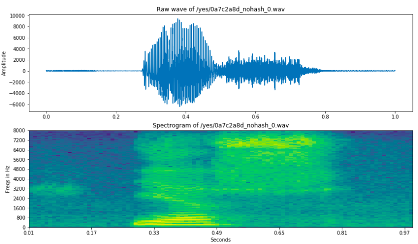

Fig.1 Raw wave and spectrogram of "yes".

Fig.1 shows the raw wave and spectrogram of "yes", respectively.

The frequencies are in range (0,8000) according to Nyquist theorem.

The codes for plotting these two figures are

freqs,times,spectrogram=log_specgram(samples,sample_rate)fig=plt.figure(figsize=(14,8))
ax1=fig.add_subplot(211)
ax1.set_title('Raw wave of '+filename)
ax1.set_ylabel('Amplitude')
ax1.plot(np.linspace(0,sample_rate/len(samples),sample_rate),samples)
ax2=fig.add_subplot(212)
ax2.imshow(spectrogram.T,aspect='auto',origin='lower',extent=[times.min(),times.max(),freqs.min(),freqs.max()])
ax2.set_yticks(freqs[::16])
ax2.set_xticks(times[::16])
ax2.set_title('Spectrogram of '+filename)
ax2.set_ylabel('Freqs in Hz')
ax2.set_xlabel('Seconds')

The spectrogram should be normalized to serve as an input features for NN

The normalization process can be realized as following example code
mean = np.mean(spectrogram, axis=0) std = np.std(spectrogram, axis=0) spectrogram = (spectrogram - mean) / std

1.2 MFCC

The tutorial for MFCC can be found in

http://practicalcryptography.com/miscellaneous/machine-learning/guide-mel-frequency-cepstral-coefficients-mfccs/

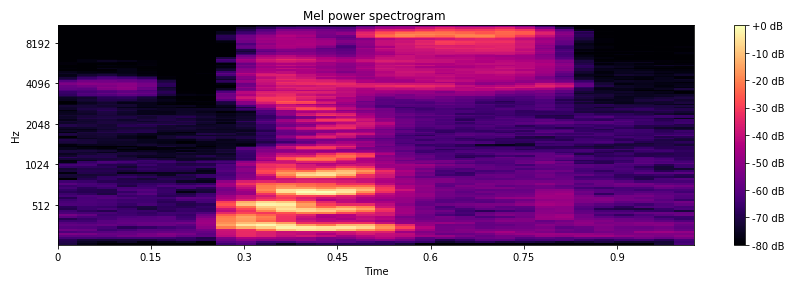Fig.2 Mel power spectrogram.

The Mel power spectrogram can be calculated using librosa python packages, and shown as Fig.2. The codes are as follows

# From this tutorial
# https://github.com/librosa/librosa/blob/master/examples/LibROSA%20demo.ipynb
S=librosa.feature.melspectrogram(samples,sr=sample_rate,n_mels=128)
# Convert to log scale (dB). We'll use the peak power (max) as reference.
log_S=librosa.power_to_db(S,ref=np.max)plt.figure(figsize=(12,4))librosa.display.specshow(log_S,sr=sample_rate,x_axis='time',y_axis='mel')
plt.title('Mel power spectrogram ')
plt.colorbar(format='%+02.0f dB')
plt.tight_layout()

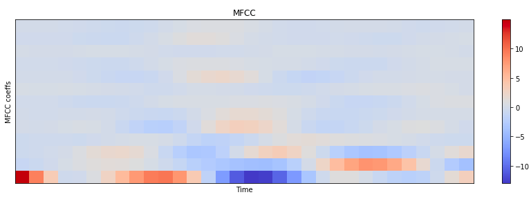
The MFCC can be calculated using librosa python packages, and shown as Fig.3. The codes are as follows

mfcc=librosa.feature.mfcc(S=log_S,n_mfcc=13)
# Let's pad on the first and second deltas while we're at it
delta2_mfcc=librosa.feature.delta(mfcc,order=2)
plt.figure(figsize=(12,4))librosa.display.specshow(delta2_mfcc)
plt.ylabel('MFCC coeffs')
plt.xlabel('Time')
plt.title('MFCC')
plt.colorbar()
plt.tight_layout()

MFCC are taken as the input tot he system instead of spectrograms in most systems.

However, in end-to-end (NN-based) systems, the most common input features are raw spectrograms, or mell power spectrograms.

MFCC decorrelates features, but NNs deal with correlated features well.

1.3 Spectrogram in 3D

The spectrogram can plotted in 3D as

(adding figure)

The codes for plotting spectrogram are as

data=[go.Surface(z=spectrogram.T)]
layout=go.Layout(
       title='Specgtrogram of "yes" in 3d',
       scene=dict(
       yaxis=dict(title='Frequencies',range=freqs),
       xaxis=dict(title='Time',range=times),
       zaxis=dict(title='Log amplitude'),
       ),
)
fig=go.Figure(data=data,layout=layout)
py.iplot(fig)

1.4 Silence removal

The file can be listen by the codes as follows

ipd.Audio(samples,rate=sample_rate)

A bit of the file from the begining and from the end can be cut, and we can listen to it again. The following codes take from 4000 to 13000:

samples_cut=samples[4000:13000]
ipd.Audio(samples_cut,rate=sample_rate)

webrtcvad package can be used to have a good Voice Activity Detection (VAD). The audio file, together with guessed alignment of 'y' 'e' 's' graphems, are ploted as

(adding) figure

The codes are as follows

freqs,times,spectrogram_cut=log_specgram(samples_cut,sample_rate)

fig=plt.figure(figsize=(14,8))
ax1=fig.add_subplot(211)
ax1.set_title('Raw wave of '+filename)
ax1.set_ylabel('Amplitude')
ax1.plot(samples_cut)
ax2=fig.add_subplot(212)
ax2.set_title('Spectrogram of '+filename)
ax2.set_ylabel('Frequencies * 0.1')
ax2.set_xlabel('Samples')
ax2.imshow(spectrogram_cut.T,aspect='auto',origin='lower',
           extent=[times.min(),times.max(),freqs.min(),freqs.max()])
ax2.set_yticks(freqs[::16])
ax2.set_xticks(times[::16])
ax2.text(0.06,1000,'Y',fontsize=18)
ax2.text(0.17,1000,'E',fontsize=18)
ax2.text(0.36,1000,'S',fontsize=18)
xcoords=[0.025,0.11,0.23,0.49]
for xc in xcoords:
    ax1.axvline(x=xc*16000,c='r')
    ax2.axvline(x=xc,c='r')