CBOW Model with One-word Context

The CBOW model predicts one word by its context words (input of CBOW model) [1].

Define a vocabulary containing $V$ words as

${\mathcal V} = \{ d_1, d_2, \cdots, d_k, \cdots, d_V\}$

where $d_k$ is the $k$-th word in the vocabulary. The training corpus ${\mathcal C}$ can be constituted by $N_a$ articles as ${\mathcal C} = \{ \textrm{article}_1, \textrm{article}_2, \cdots, \textrm{ article}_{N_a} \}$.

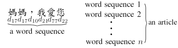
Fig.1. Schematic of a word sequence and an article.

Fig.1. shows the schematic of a word sequence and an article. A word sequence is formed by concatenating the words in the vocabulary ${\mathcal V}$. Each article is formed by concatenating $n$ word sequences.

Considering the context word being one word, the CBOW is reduced to a bigram model.

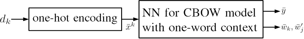Fig.2. Data flow of CBOW model with one-word context.$\bar{x}^k$ is the one-hot encoded vector of word $d_k$ and is input to the NN for CBOW model with one-word context. $\bar{y}$ is the output of the NN. The input word vector representation $\bar{w}_k$ and output word vector representation $\bar{w}_j'$ are two kinds of word vector representations.

Fig.2. shows the data flow of CBOW model with one-word context.The word $d_k$ is one-hot encoded into $\bar{x}^k$ and $\bar{x}^k$ is input to the neural network (NN) for CBOW model with one-word context, expanded as

$\bar{x}^k = [x_1^k, x_2^k, \cdots, x_{k-1}^k, x_k^k, x_{k+1}^k, \cdots, x_V^k]^t \pod{\text{1}}$

where $x_n^k = 0$ for $n \neq k$ and $x_k^k = 1$; $t$ stands for transpose operation.

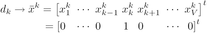
Fig.3 Schematic of one-hot encoding for $k$-th word, $d_k \to \bar{x}^k = [x_1^k, x_2^k,\cdots, x^k_k,\cdots, x_V^k]^t=[0,\cdots, 1, \cdots, 0]^t$

Fig.3 shows the schematic of one-hot-encoding for $k$-th word $d_k$.

The output $\bar{y} = [y_1, \cdots, y_j, \cdots, y_V]^t$ has the size of $V$; $y_j = p(d_j| \bar{x}^k)$ is a probability that the next word is $d_j$ given the one-hot encoded vector $\bar{x}^k$ with the property that $\displaystyle \sum_{j=1}^V y_j=1$.

The NN is trained by inputting the articles in the training corpus ${\mathcal C}$ to the NN word by word with the given context word $d_k$ and its corresponding target word $d_{j_t}$. $j_t$ is the index of the target word.

Fig.4 Schematic of the target word $d_{j_t}$ under CBOW model of one-word context $d_k$. (a) $d_k = d_{17}$, $d_{j_t} = d_{17}$. (b) $d_k = d_{21}$, $d_{j_t} = d_{77}$.

Fig.4 shows the schematic of the target word under CBOW model of one-word context. The target word is the next word of the given context word in the word sequence.

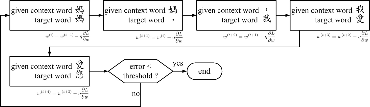Fig.5. Overall training flow-chart of the example "媽媽，我愛您".

Fig.5 shows the overall training flow-chart of the example "媽媽，我愛您".

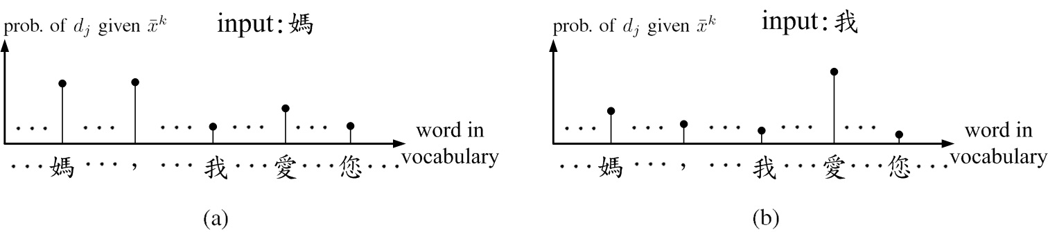Fig.6. Schematic of output $\bar{y}$ of a well-trained NN given $\bar{x}^k$ in a testing example. (a) input "媽", (b) input "我".

Fig.6 shows the schematic of output $\bar{y}$ of a well-trained NN given $\bar{x}^k$ in a testing example for input words "媽" and "我". As testing a well-trained NN with input word "媽", one finds that the probabilities of "媽" and "，" might be higher than most other words in the vocabulary. As inputting "我", the probability of "愛" might be higher than most other words in the vocabulary.

The input word vector representation $\bar{w}_k$ and output word vector representation $\bar{w}_j'$ are two kinds of word vector representations.

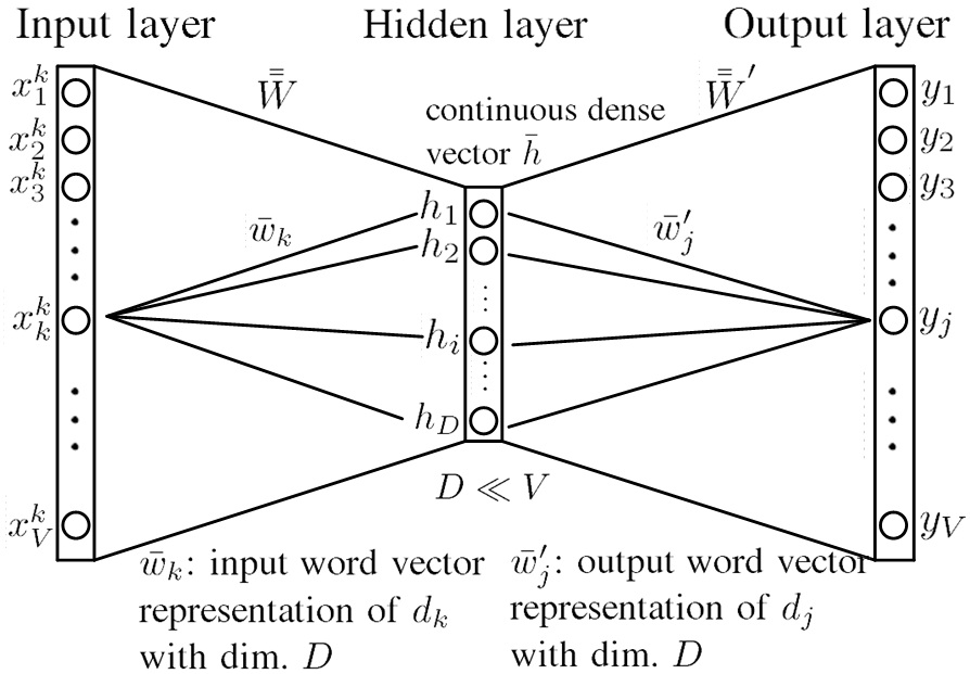
Fig.7. Architecture of the NN for the CBOW model with one context word. $\bar{w}_k$ is input word vector representation of $d_k$, and $\bar{w}_j'$ is output word vector representation of $d_j$. Both of $\bar{w}_k$ and $\bar{w}_j'$ are of dimension $D$, $D \ll V$.

Fig.7 shows the architecture of the NN for the CBOW model with one context word.$\bar{\bar{W}}$ and $\bar{\bar{W}}'$ are the input-to-hidden and hidden-to-output weight matrices. $\bar{w}_k$ is input word vector representation of $d_k$ and $\bar{w}_j'$ is output word vector representation of $d_j$. The neuron numbers in the input layer and in the output layer are both chosen to be the vocabulary size $V$, and the hidden layer size is $D$. Usually, $D \ll V$. For example, $V = 8000$ and $D = 60$ or $100$.

Forward Propagation

The input-to-hidden weight between the neuron $k$ in the input layer and the neuron $i$ in the hidden layer is denoted as $w_{ki}$ , forming a $V \times D$ weight matrix as

$\bar{\bar{W}} = \left[\begin{matrix} w_{11} & w_{12} & \cdots & \cdots & w_{1D} \\ w_{21} & w_{22} & \cdots& \cdots & w_{2D} \\ \vdots & \cdots & \ddots& \cdots & \vdots \\ w_{k1} & \cdots & w_{ki}& \cdots & w_{kD} \\ \vdots & \cdots & \ddots& \cdots & \vdots \\ w_{V1} & w_{V2} & \cdots & \cdots & w_{VD} \end{matrix}\right] \pod{\text{2}}$

where the $k$-th row of $\bar{\bar{W}}$ contains the weights whcih connect the neuron $k$ in the input layer to all neurons in the hidden layer as shown in Fig.6. Define the transpose of the $k$-th row of $\bar{\bar{W}}$ as the input word vector representation $\bar{w}_k$, namely,

$\bar{w}_{k} \doteq \left[ \begin{matrix} w_{k1}, \cdots, w_{ki}, \cdots, w_{kD} \end{matrix} \right]^t$

which is the $D$-dimensional vector representation of the input word $d_k$.

The hidden-layer output is obtained as

$\bar{h} = \bar{\bar{W}}^{t}\bar{x}^{k}$

$=\left[\begin{matrix} w_{11} & w_{21} & \cdots & w_{k1} & \cdots & w_{V1} \\ w_{12} & w_{22} & \cdots & \cdots & \cdots & w_{V2} \\ \vdots & \cdots & \cdots & w_{ki}& \cdots & \vdots \\ \vdots & \cdots & \ddots& \cdots & \vdots & \vdots \\ w_{1D} & w_{2D} & \cdots & w_{kD} & \cdots & w_{VD} \end{matrix}\right] \left[\begin{matrix} 0 \\ \vdots \\ 0 \\ x_k^k = 1 \\ 0 \\ \vdots \\ 0 \end{matrix}\right] = \left[\begin{matrix} w_{k1} \\ \vdots \\ w_{ki} \\ \vdots \\ w_{kD} \end{matrix}\right] = \bar{w}_{k} \pod{\text{3}}$

The hidden-to-output weights are denoted as $w_{ij}'$, which connect the neuron $i$ in the hidden layer and the neuron $j$ in the output layer and form an $D \times V$ weight matrix $\bar{\bar{W}}'$ as

$\bar{\bar{W}}' = \left[ \begin{matrix} w_{11}' & w_{12}' & \cdots & w_{1j}' & \cdots & w_{1V}' \\ w_{21}' & w_{22}' & \cdots & w_{2j}'& \cdots & w_{2V}' \\ \vdots & \cdots & \ddots & \cdots & \cdots & \vdots \\ w_{i1}' & \cdots & \cdots & w_{ij}' & \cdots & w_{iV}' \\ \vdots & \cdots & \ddots & \cdots & \cdots & \vdots \\ w_{D1}' & w_{D2}' & \cdots & w_{Dj}' & \cdots & w_{DV}' \end{matrix} \right] \pod{\text{4}}$

where the $j$-th column contains the weights which connect all neurons in the hidden layer to the $j$-th neuron in the output layer as shown in Fig.2. Define the $j$-th column of $\bar{\bar{W}}'$ as the output vector $\bar{v}_j'$, namely,

$\bar{w}_j' \doteq [w_{1j}', w_{2j}', \cdots, w_{ij}', \cdots, w_{Dj}']^t \pod{\text{5}}$

Note that the output vector $\bar{w}_k'$ is another $D$-dimensional vector representation of the input word $d_k$. By substituting $(5)$ into $(4)$, we can represent $\bar{\bar{W}}'$ as

$\bar{\bar{W}}' = \left[ \bar{w}'_1, \cdots, \bar{w}'_j, \cdots, \bar{w}'_V \right] \pod{\text{6}}$

The vector $\bar{h}$ in $(3)$ is weighted by $\bar{\bar{W}}'$ to obtain the input of the output layer as

$\bar{u} = {\bar{\bar{W}}'}^t \cdot \bar{h} = \left[ \begin{matrix} w_{11}' & w_{21}' & \cdots & w_{i1}' & \cdots & w_{D1}' \\ w_{12}' & w_{22}' & \cdots & \vdots & \cdots & w_{D2}' \\ \vdots & \vdots & \ddots & w_{ij}' & \cdots & \vdots \\ \vdots & \vdots & \vdots & \vdots & \ddots & \vdots \\ w_{1V}' & w_{2V}' & \cdots & w_{iV}' & \cdots & w_{DV}' \end{matrix} \right] \left[ \begin{matrix} w_{k1} \\ \vdots \\ w_{ki} \\ \vdots \\ w_{kD} \end{matrix} \right] = \left[ \bar{w}'_1, \cdots, \bar{w}'_j, \cdots, \bar{w}'_V \right]^t \bar{w}_k$

which can be represented as

$\bar{u} = \left[ \bar{w}'_1, \cdots, \bar{w}'_j, \cdots, \bar{w}'_V \right]^t \bar{w}_k = \left[ \begin{matrix} u_1 \\ \vdots \\ u_j \\ \vdots \\ u_V \end{matrix} \right] = \left[ \begin{matrix} {\bar{w}_1'}^t \bar{w}_k \\ \vdots \\ {\bar{w}_j'}^t \bar{w}_k \\ \vdots \\ {\bar{w}_V'}^t \bar{w}_k \end{matrix} \right] = \left[ \begin{matrix} \bar{w}_1' \cdot \bar{w}_k \\ \vdots \\ \bar{w}_j' \cdot \bar{w}_k \\ \vdots \\ \bar{w}_V' \cdot \bar{w}_k \end{matrix} \right] \pod{\text{7}}$

The output $y_j$ of the $j$-th neuron in the output layer is a probability that the next word is $d_j$ given the one-hot encoded vector $\bar{x}^k$ as

$y_j = p(d_j | \bar{x}^k)= \frac{e^{u_j}}{\displaystyle \sum_{j = 1}^V e^{u_j}} = \frac{e^{\bar{w}'_j \cdot \bar{w}_k}}{\displaystyle \sum_{j = 1}^V e^{\bar{w}'_j \cdot \bar{w}_k}} \pod{\text{8}}$

The training objective is to maximize the probability $y_{j_t}$ of observing the target word $d_{j_t}$ given $\bar{x}^k$.

The loss function is defined as

$L = -\ln p(d_{j_t} | \bar{x}^k) \pod{\text{9}}$

Note that maximizing $y_{j_t} = p(d_{j_t} | \bar{x}^k)$ is to minimize $L$.

Backward Propagation

By using $(8)$, the loss function is expressed as

$L = -\ln y_{j_t} = - u_{j_t} + \ln \left(\sum_{j=1}^V e^{u_j} \right) \pod{\text{10}}$

The partial derivative of $L$ with respect to $u_j$ is

$\frac{\partial L}{\partial u_j} = y_j - \hat{y}_j \pod{\text{11}}$

where we define the desired output $\hat{y}_j$ as

$\hat{y}_j = \left\{ \begin{matrix} 0, & j \neq j_t \\ 1, & j = j_t \end{matrix} \right.$

The supporting material of $(11)$ is

$\begin{aligned} & \frac{\partial L}{\partial u_{j_t}} = -1 + \frac{e^{u_{j_t}} }{\displaystyle \sum_{j=1}^V e^{u_j}} = y_{j_t} - 1 \\ & \frac{\partial L}{\partial u_j} = \frac{\partial L}{\partial y_{j_t}} \frac{\partial y_{j_t}}{\partial u_j} = - \frac{1}{y_{j_t}}\frac{\partial y_{j_t}}{\partial u_j}= -\frac{1}{y_{j_t}} \frac{\partial \frac{e^{u_{j_t} }}{\sum_{j=1}^V e^{u_j}}}{\partial u_j} =-\frac{1}{y_{j_t}} e^{u_{j_t}} \frac{\partial \displaystyle \left( \sum_{j=1}^V e^{u_j} \right)^{-1}}{ \partial u_j} \\ &= -\frac{1}{y_{j_t}} e^{u_{j_t}} \left[-\left( \sum_{j=1}^V e^{u_j} \right)^{-2} \right] \frac{ \partial \left( \sum_{j=1}^V e^{u_j} \right) }{\partial u_j} \\ &= \frac{1}{y_{j_t}} \frac{e^{u_{j_t}} }{ \sum_{j=1}^V e^{u_j} } \frac{e^{u_j} }{ \sum_{j=1}^V e^{u_j} } = \frac{y_{j_t}}{y_{j_t}} y_j = y_j, \ j \neq j_t \end{aligned}$

Thus, we can define the error between the NN output and the desired output as

$\bar{e} = \bar{y} - \hat{y} \ \mathrm{or} \ e_j = y_j - \hat{y}_j \pod{\text{12}}$

where $\hat{y} = [\hat{y}_1, \cdots, \hat{y}_j, \cdots, \hat{y}_V]^t$.

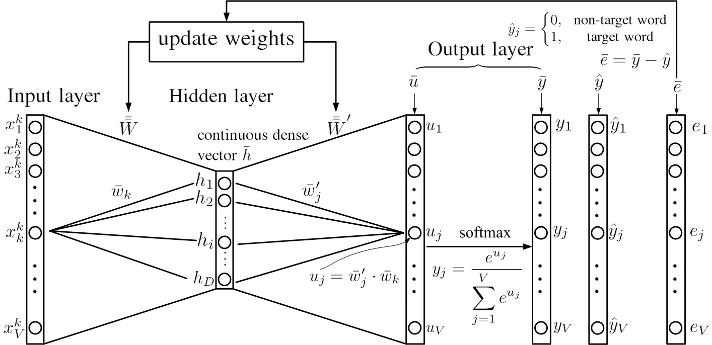Fig.8. Overview of updating weights of the NN for CBOW model.

Fig.8 shows the overview of updating weights of the NN for CBOW model.

The derivative of $L$ to the hidden-to-output weight $w_{ij}'$ is

$\frac{\partial L}{\partial w'_{ij}} = \frac{\partial L}{\partial u_j} \frac{\partial u_j}{\partial w'_{ij}} = e_j w_{ki} \pod{\text{13}}$

The supporting material of $(13)$ is

$\begin{aligned} u_j = \bar{w}_j' \cdot \bar{w}_k & = \sum_{i = 1}^N w_{ij}' w_{ki} \\ \frac{\partial u_j}{\partial w'_{ij}} & = w_{ki} \end{aligned}$

By using stochastic gradient descent, we obtain the updating equation for hidden-to-output weights $w_{ij}'$ as

${w_{ij}'}^{(new)} = {w_{ij}'}^{(old)} - \eta \frac{\partial L}{\partial w'_{ij}} = {w_{ij}'}^{(old)} - \eta e_j w_{ki}^{(old)} \pod{\text{14}}$

or equivalently

${\bar{w}_j'}^{(new)} = {\bar{w}_j'}^{(old)} - \eta e_j \bar{w}_k^{(old)} \pod{\text{15}}$

where $\eta > 0$ is the learning rate.

Since at $j \neq j_t$, $e_j > 0$, which is called overestimating and can be seen in $(12)$, that ${\bar{w}_j'}^{(old)}$ subtract a scaled $\bar{w}_k^{(old)}$ in $(15)$ leads to the angle between ${\bar{w}_j'}^{(new)}$ and $\bar{w}_k^{(old)}$ increasing. Since at $j = j_t$, $e_j < 0$, which is called underestimating, that ${\bar{w}_j'}^{(old)}$ add a scaled $\bar{w}_k^{(old)}$ in $(15)$ leads to the angle between ${\bar{w}_j'}^{(new)}$ and $\bar{w}_k^{(old)}$ decreasing. If $y_{j_t}$ is close to 1, the error is close to 0 and $\bar{w}'_{j_t}$ is nearly unchanged.

Next, find the update equation for input-to-hidden weights $\bar{\bar{W}}$. The derivative of $L$ to the output of the hidden layer $h_i$ is

$\frac{\partial L}{\partial h_i} = \sum_{j = 1}^V \frac{\partial L}{\partial u_j} \frac{\partial u_j}{\partial h_i} = \sum_{j = 1}^V e_j w'_{ij} \pod{\text{16}}$

The supporting material of $(16)$ is

$h_i = w_{ki}$

and

$\frac{\partial u_j}{\partial h_i} = \frac{\partial u_j}{\partial w_{ki}} = w_{ij}'$

The derivative of $L$ to the input-to-hidden weights $w_{ki}$ is

$\frac{\partial L}{\partial w_{ki}} = \frac{\partial L}{\partial h_i} \frac{\partial h_i}{\partial w_{ki}} = \frac{\partial L}{\partial h_i} = {\displaystyle \sum_{j = 1}^V} e_j w'_{ij} \pod{\text{17}}$

The update equation for input-to-hidden weights $w_{ki}$ is

$w_{ki}^{(new)} = w_{ki}^{(old)} - \eta \frac{\partial L}{\partial w_{ki}} = w_{ki}^{(old)} - \eta \sum_{j = 1}^V e_j {w_{ij}'}^{(old)} \pod{\text{18}}$

or

$\bar{w}_k^{(new)} = \bar{w}_k^{(old)} - \eta \sum_{j = 1}^V e_j {\bar{w}_j'}^{(old)} \pod{\text{19}}$

The input word vector representation $\bar{w}_k$ is updated by adding the sum of scaled output word vector representations $\bar{w}_j'$. At $j \neq j_t$ ($e_j > 0$) , the contribution of $\bar{w}_j'$ will put $\bar{w}_k$ farther away from $\bar{w}_j'$. At $j = j_t$ ($e_j < 0$), the contribution of $\bar{w}_{j_t}'$ will move $\bar{w}_k$ closer to $\bar{w}_{j_t}'$. If the contribution of all the output word vectors is nearly zero, the input word vector remains nearly unchanged.

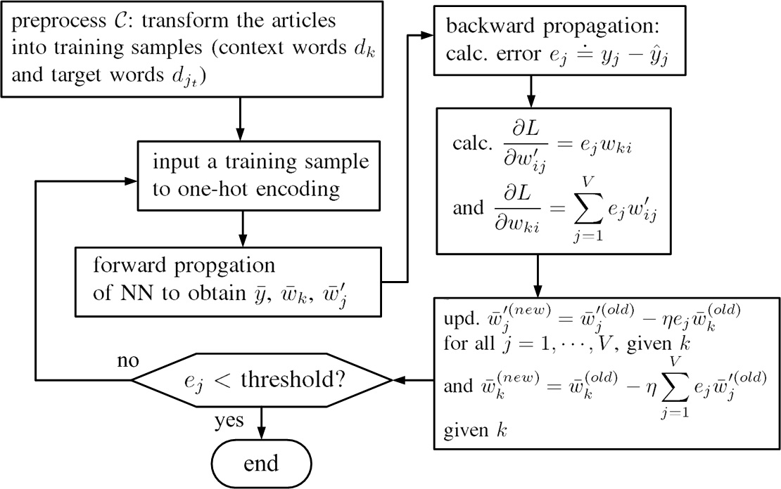Fig.9. Flow-chart to train distributed vector representations of words in vocabulary ${\mathcal V}$ by a training corpus ${\mathcal C}$.

Fig.9. shows a flow-chart to train distributed vector representations of words in vocabulary ${\mathcal V}$ by a training corpus ${\mathcal C}$.

[0]

X. Rong, word2vec parameter learning explained, arXiv:1411.2738, 2014.

[1]

T. Mikolov, K. Chen, G. Corrado and J. Dean, Efficient estimation of word representations in vector space,

arXiv:1301.3781, 2013.