Optimization

Machine Learning Model

Fig.1 Schematic of Machine learning model, label data and loss function $L$.

Fig.1 shows the schematic of machine learning model, label data $\hat{y}$ and loss function $L$.

The machine learning model are characterized by the weight $\bar{\bar{w}}$ and bias $\bar{b}$.

$\bar{x}$ is the input data, and $\bar{y}$ is the output data. $\bar{y}$ can be also seen as the model prediction.

$\hat{y}$ is the label data. Loss function measure the distance between model prediction $\bar{y}$ and label data $\hat{y}$.

The target of machine learning is to find the model (usually characterized with $\bar{\bar{w}}$ and $\bar{b}$) with the model prediction $\bar{y}$ close to $\hat{y}$.

In other words to minimize the loss function value $L$.

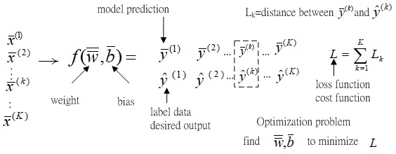
Fig.2 schematic of Machine learning frame work as an optimization problem.

Fig.2 shows the schematic of machine learning frame work as an optimization problem.

$\bar{x}^{(1)},\bar{x}^{(2)},\cdots, \bar{x}^{(k)}, \cdots, \bar{x}^{(K)}$are K dataset, and $\bar{y}^{(1)},\bar{y}^{(2)},\cdots, \bar{y}^{(k)}, \cdots, \bar{y}^{(K)}$are its corresponding model predictions.

$\hat{y}^{(1)},\hat{y}^{(2)},\cdots, \hat{y}^{(k)}, \cdots, \hat{y}^{(K)}$are the corresponding label datum.

$L_k$ refers to the distance between the $k$th model prediction $\bar{y}^{(k)}$ and label data $\hat{y}^{(k)}$.

The loss function $L$ is defined as the over all $K$ data, $L=\displaystyle \sum_{k=1}^K L_k$.

The machine learning can be seen as the optimization problem:

Find $\bar{\bar{w}}$ s and $\bar{b}$ to minimize the loss function value $L$.

$\bar{\bar{w}},\bar{b} = \displaystyle \min_{\bar{\bar{w}},\bar{b} } L$

The gradient descent is applied to solve this optimization problem.

Gradient descent

The update rule based on gradient descent can be expressed as

$w^{(t)}=w^{(t-1)} - \eta \frac{\partial L}{\partial w}$.

where $\eta$ is the learning rate.

One dimension example

Assuming the loss function is obtained as $L(w)=w^2$, we can derive $\frac{\partial L}{\partial w}=2 w$.

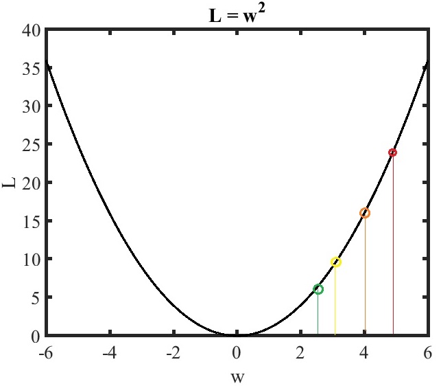
Fig.3 Gradient decent example 1 with $\eta=0.1$.

If $w$ is initialized as 5, $w^{(t=0)}=5$, we derive $\frac{\partial L}{\partial w}= 2 w^{(0)}= 2 \times 5 =10$.

Assuming the learning rate $\eta$=0.1, the w at time 1,$t=1$, is updated as

$w^{(1)}=w^{(0)}-0.1 \times 2 \times 5 =5-1=4$

the w at time 2,$t=2$, is updated as

$w^{(2)}=w^{(1)}-0.1 \times 2 \times 4=4-0.8=3.2$

the w at time 3,$t=3$, is updated as

$w^{(3)}=w^{(2)}-0.1 \times 2 \times 3.2=3.2-0.64=2.56$

As time goes infinity, the $w^{(t \to \infty)}=0$.

considering larger learning rate

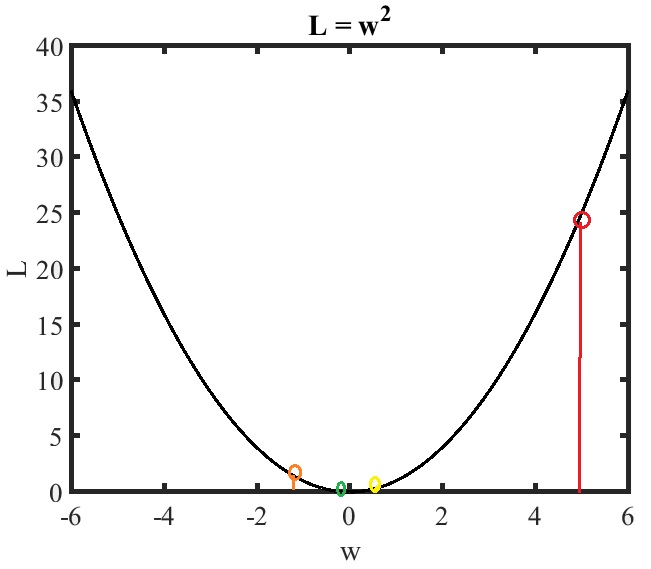
Fig.4 Gradient decent example 1 with $\eta=0.6$.

Considering a larger learning rate $\eta=0.6$,

the w at time 1,$t=1$, is updated as

$w^{(1)}=w^{(0)}-0.6 \times 2 \times 5 =5-6=-1$

the w at time 2,$t=2$, is updated as

$w^{(2)}=w^{(1)}-0.6 \times 2 \times (-1) =(-1)-(-1.2) =0.2$

the w at time 3,$t=3$, is updated as

$w^{(3)}=w^{(2)}-0.6 \times 2 \times (0.2)=0.2-0.24=-0.04$

As time goes infinity, the $w^{(t \to \infty)}=0$.

The convergence rate with $\eta=0.6$ is larger than that with $\eta=0.1$ in this illustrative example.

considering a even larger learning rate

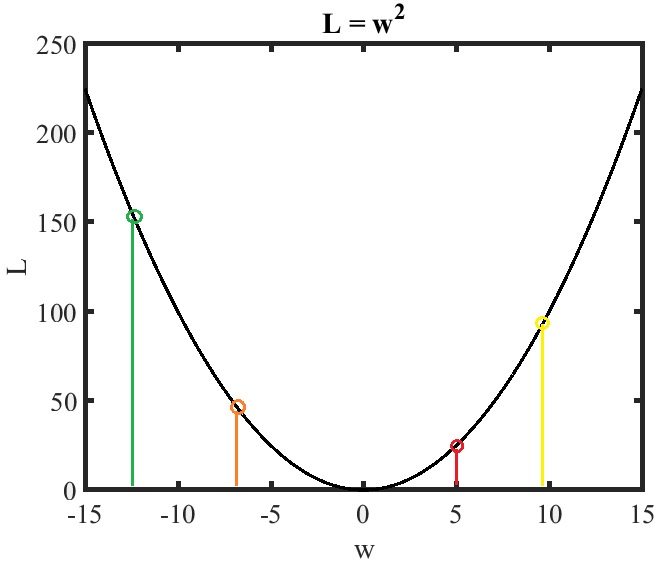
Fig.5 Gradient decent example 1 with $\eta=1.2$.

Considering a even larger learning rate $\eta=1.2$,

the w at time 1,$t=1$, is updated as

$w^{(1)}=w^{(0)}-1.2 \times 2 \times 5 =5-12=-7$

the w at time 2,$t=2$, is updated as

$w^{(2)}=w^{(1)}-1.2 \times 2 \times (-7) =(-7)-(-16.8) =9.8$

the w at time 3,$t=3$, is updated as

$w^{(3)}=w^{(2)}-1.2 \times 2 \times (9.8)=9.8-23.52=-13.72$

As time goes infinity, the $w^{(t \to \infty)}$.will diverge.