Back propagation

Back propagation是一種有效率算出$\frac{\partial{L}}{\partial{\bar{\bar{W}}}}$ 來讓訓練Neural Network變得更有效率。

一個Neural Network裡可能有上百萬的參數(weights $\bar{\bar{W}}$, biases $\bar{b}$)，在使用Gradient Descent作訓練時就會產生上百萬維的矩陣 $\partial{L} \over \partial{\bar{\bar{W}}}$ 和 $\partial{L} \over \partial{\bar{\bar{b}}}$，其中$L$ 是loss function，如下圖一所示:

圖一 Overview of Gradient Descent.

圖二.機器學習的Forward propagation and backward propagation 的示意圖。

圖二呈現機器學習的Forward propagation and backward propagation 示意圖，forward propagation指的是順向運算，意義上是機器

做出推論。backward propagation指的是逆向運算，意義上是學習，本質是調整機器的參數($\bar{\bar{w}}$,$\bar{b}$)。其實，當Forward propagation 清楚定義後，Back propagation 也已經被決定。 Tensorflow會幫忙計算 Back propogation 中複雜的$\frac{\partial{L}}{\partial{\bar{w}}}$

Back propagation立基於微積分的Chain rule，如下圖三所示:

圖三 Schematic of Chain Rule

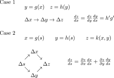
考慮 $y$ 是 $x$的函數，而 $z$ 是$y$ 的函數，當$x$有$\Delta x$ 變化時，$z$將有$\Delta z$的變化。將$z$對$x$微分的定義是：

$\begin{aligned} \frac{\partial z}{\partial x} = \mathop {\lim }\limits_{\Delta x \to 0}{\frac{\Delta z}{\Delta x}} = \frac{\partial z}{\partial y} \frac{\partial y}{\partial x} = h'g' \end{aligned}$

先看下圖四的一個Neural Network，輸入K筆input data: x，

會得到K筆output data: y，而$L_k$是每一筆輸出output data與label data的距離。

$L_k(\bar{\bar{w}},\bar{b})=\textrm{distance}(\bar{y},\hat{y})$

定義Loss function為每筆data 的L值總合。

$L=\sum_{k=1}^K L_k$

計算Loss function對其中一變數w偏微分時即是L值總合對變數w偏微分。

$\frac{\partial L}{\partial w}=\sum_{k=1}^k \frac{\partial L_k}{\partial w}$

圖四 Neural Network, loss function, and weight gradient of loss function

以圖四中Loss 對w作偏微分為範例，其等於z對w作偏微分乘上Loss對z偏微分。其中z對w作偏微分稱作forward pass，Loss對z偏微分稱作backward pass。z 為activation function 的input。

圖五 Forward pass and backward pass of weight gradient $\frac{\partial L}{\partial \bar{\bar{w}}}$ computation

Forward Pass

先看forward pass: z對w作偏微分 如下圖五 z對w作偏微分即為input x

圖六 Elaboration on forward pass of $\frac{\partial L}{\partial w}$ computation

Backward pass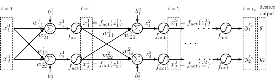

圖七. 深層神經網絡架構之訓練(deep neural network, DNN)。網絡層數為$\ell_e$， 第$\ell$層之神經元數為$D_\ell = 2$，其神經元表示為$\bar{x}^\ell$，激活函數為$f_{\mathrm act}$，渴望輸出(desired output)為$\bar{y} = [y_1, y_2]^t$。

圖七顯示深層神經網絡架構之訓練。網絡層數為$\ell_e$， 第$\ell$層神經元數為$D_\ell = 2$，其神經元表示為$\bar{x}^\ell$，激活函數為$f_{\mathrm act}$，渴望輸出(desired output)為$\bar{y} = [y_1, y_2]^t$，$t$為轉置操作。

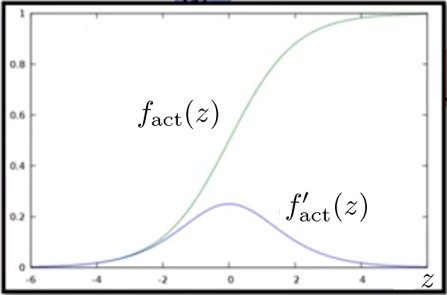
圖八. 激活函數$f_{\mathrm act}$與其導函數$f_{\mathrm act}'$。此處激活函數選為sigmoid function。

圖八顯示激活函數$f_{\mathrm act}$與其導函數$f_{\mathrm act}'$。此處激活函數選為sigmoid function。

考慮第$\ell$層，此層輸入$\bar{x}^{\ell-1}$(為前一層神經元)與此層神經元$\bar{x}^\ell$間之權重矩陣以及偏差表示為

$\bar{\bar{W}}^\ell = \left[ \begin{matrix} w_{11}^\ell & w_{12}^\ell \\ w_{21}^\ell & w_{22}^\ell \end{matrix} \right], \ \bar{b}^\ell = \left[ \begin{matrix} b_1^\ell \\ b_2^\ell \end{matrix} \right] \pod{\text{1}}$

激活函數輸入值$\bar{z}^\ell$為第$\ell-1$層神經元乘以權重矩陣之轉置加上偏差而得，即

$\bar{z}^\ell = \bar{\bar{W}}^{\ell t} \bar{x}^{\ell - 1} + \bar{b}^\ell = \left[ \begin{matrix} z_1^\ell \\ z_2^\ell \end{matrix} \right] = \left[ \begin{matrix} w_{11}^\ell & w_{21}^\ell \\ w_{12}^\ell & w_{22}^\ell \end{matrix} \right] \left[ \begin{matrix} x_1^{\ell-1} \\ x_2^{\ell-1} \end{matrix} \right] + \left[ \begin{matrix} b_1^\ell \\ b_2^\ell \end{matrix} \right]\pod{\text{2}}$

Backward pass所要求的目標是損耗函數$L$對激活函數輸入值$z_n^\ell$($n = 1,2$)的偏導數，此項目稱為error sensitivity，即

$\displaystyle \frac{\partial L}{\partial z_n^\ell} = \frac{\partial L}{\partial x_n^\ell} \frac{\partial x_n^\ell}{\partial z_n^\ell} = \frac{\partial L}{\partial x_n^\ell} f'_{\mathrm act}(z_n^\ell) \pod{\text{3}}$

其中，由圖七可看出$x_n^\ell = f_{\mathrm act}(z_n^\ell)$。而$L$對神經元$x_n^\ell$的偏導數可再由$\ell+1$層的error sensitivity表達，即

$\frac{\partial L}{\partial x_n^\ell} = \sum_{m = 1}^{D_{\ell+1} = 2} \frac{\partial L}{\partial z_m^{\ell+1}} \frac{\partial z_m^{\ell+1}}{\partial x_n^\ell} = \sum_{m = 1}^{D_{\ell+1} = 2} \frac{\partial L}{\partial z_m^{\ell+1}} w_{nm}^{\ell+1} \pod{\text{4}}$

以第一層$\ell= 1$為例，網絡輸入$\bar{x}^0$(可視為第零層神經元)與第一層神經元$\bar{x}^1$間之權重矩陣以及偏差表示為

$\bar{\bar{W}}^1 = \left[ \begin{matrix} w_{11}^1 & w_{12}^1 \\ w_{21}^1 & w_{22}^1 \end{matrix} \right], \ \bar{b}^1 = \left[ \begin{matrix} b_1^1 \\ b_2^1 \end{matrix} \right] \pod{\text{5}}$

激活函數輸入$\bar{z}^1$為第零層神經元乘以權重矩陣之轉置加上偏差而得，即

$\bar{z}^1 = \bar{\bar{W}}^{1t} \bar{x}^0 + \bar{b}^1 = \left[ \begin{matrix} z_1^1 \\ z_2^1 \end{matrix} \right] = \left[ \begin{matrix} w_{11}^1 & w_{21}^1 \\ w_{12}^1 & w_{22}^1 \end{matrix} \right] \left[ \begin{matrix} x_1^0 \\ x_2^0 \end{matrix} \right] + \left[ \begin{matrix} b_1^1 \\ b_2^1 \end{matrix} \right]\pod{\text{6}}$

損耗函數$L$對激活函數輸入值$z_1^1$的偏導數為

$\displaystyle \frac{\partial L}{\partial z_1^1} = \frac{\partial L}{\partial x_1^1} \frac{\partial x_1^1}{\partial z_1^1} = \frac{\partial L}{\partial x_1^1} f_{\mathrm act}'(z_1^1) \pod{\text{7}}$

其中

$\displaystyle \frac{\partial L}{\partial x_1^1} = \frac{\partial z_1^2}{\partial x_1^1} \frac{\partial L}{\partial z_1^2} +\frac{\partial z_2^2}{\partial x_1^1}\frac{\partial L}{\partial z_2^2}$

$\frac{\partial L}{\partial x_1^1} = w_{11}^2 \frac{\partial L}{\partial z_1^2} + w_{12}^2 \frac{\partial L}{\partial z_2^2} \pod{\text{8}}$

圖九. 第一層神經元$x_1^1$與第二層神經元之連結。

圖九顯示第一層神經元$x_1^1$與第二層神經元之連結。當$L$要對$x_1^1$做偏微分時，依chain rule會先微至$z_n^2$($n = 1,2$)，得出error sensitivity，再參考圖九，得出$(8)$。

圖十.反向網絡。輸入為error sensitivity。網絡結構與圖九網絡相同，權重亦相同。

圖十顯示一反向網絡。輸入為error sensitivity。網絡結構與圖九網絡相同，權重亦相同。式$(8)$可看成一個反向網絡如圖十，結構與權重均與原網絡相同，唯傳播方向相反。

最後，backpropagation的目標，$L$對權重的偏導數，即為forward pass與backward pass兩者所得結果之乘積，

$\frac{\partial L}{\partial w_{nm}^\ell} = \frac{\partial L}{\partial z_n^\ell} \frac{\partial z_n^\ell}{\partial w_{nm}^\ell} \pod{\text{9}}$