initialize parameters

Initialize parameters is the "Similarity Mapping Layer" part of QACNN model.

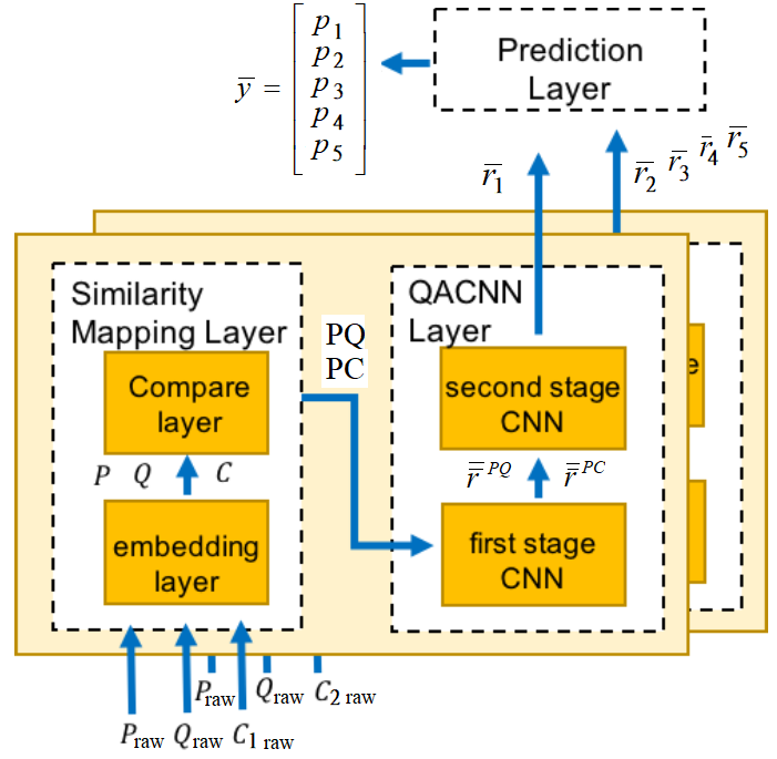
Fig.1 Overall data flow of QACNN model

# initialize parameter分成兩個部分，第一部分是12~35行, 將建構 "embedding layer"，第二部分是38~48行, 將建構 "Compare layer"。

The embedding layer transform $P_{raw}$, $Q_{raw}$,
$C\_{raw}$ into word embedding $P$, $Q$, and $C$.

The compare layer generates paragraph-query similarity map $PQ$ and paragraph-choice similarity map $PC$.

# initialize parameter

Given a paragraph $P_{\textrm{raw}}$ (with $N$ sentences), a query $Q_{\textrm{raw}}$, and a choice $C_{\textrm{raw}}$, the embedding layer transforms every words in $P_{\textrm{raw}}$, $Q_{\textrm{raw}}$ and $C_{\textrm{raw}}$ into word embedding, whose length is x_dimension.
$P =\{\bar{p}_n^i \}_{i=1,n=1}^{I,N}$ $\colon$ $N$ is the total number of sentence in paragraph, and $I$ is the total number of words in each sentence.

$Q =\{\bar{q}^j \}_{j=1}^{J}$ $\colon$ Query is considered as one sentence.

$J$ is the total number of words in query sentence.

$\bar{C}=\{\bar{c}^k\}^K_{k=1}$ $\colon$ choice is considered as one sentence.

$K$ is the total number of words in choice sentence.

The sentences in all the paragraphs have the same length by padding.

$\bar{p}_n^i$, $\bar{q}^i$ and $\bar{c}^k$ are word embeddings.

The compare layer compares each paragraph sentence $P_n$ to $Q$ and $C$ at word level separately.

__init__() 函數中， # initialize parameters # 第一部分為以下 12~35 行 :

12  def __init__(self,batch_size,x_dimension,dnn_width,cnn_filterSize,cnn_filterSize2,cnn_filterNum,cnn_filterNum2 ,learning_rate,dropoutRate,choice,max_plot_len,max_len,parameterPath):
13      self.parameterPath = parameterPath
14      self.p = tf.placeholder(shape=(batch_size,max_plot_len,max_len[0],x_dimension), dtype=tf.float32) ##(batch_size,p_sentence_num,p_sentence_length,x_dimension)
15      self.q = tf.placeholder(shape=(batch_size,max_len[1],x_dimension), dtype=tf.float32) ##(batch_size,q_sentence_length,x_dimension)
16      self.ans = tf.placeholder(shape=(batch_size*choice,max_len[2],x_dimension), dtype=tf.float32) ##(batch_size*5,ans_sentence_length,x_dimension)
17      self.y_hat = tf.placeholder(shape=(batch_size,choice), dtype=tf.float32) ##(batch_size,5)
18      self.dropoutRate = tf.placeholder(tf.float32)
19      self.filter_size = cnn_filterSize
20      self.filter_size2 = cnn_filterSize2
21      self.filter_num = cnn_filterNum
22      self.filter_num2 = cnn_filterNum2
23      choose_sentence_num = max_plot_len    
24    
25
26      normal_p = tf.nn.l2_normalize(self.p,3)
27      ## (batch_size,max_plot_len*max_len[0],x_dimension)
28      normal_p = tf.reshape(normal_p,[batch_size,max_plot_len*max_len[0],x_dimension])
29    
30      ## (batch_size,max_len[1],x_dimension)
31      normal_q = tf.reshape(tf.nn.l2_normalize(self.q,2),[batch_size,max_len[1],x_dimension])
32    
33      normal_ans = tf.nn.l2_normalize(self.ans,2)
34      ## (batch_size,choice*max_len[2],x_dimension)
35      normal_ans = tf.reshape(normal_ans,[batch_size,choice*max_len[2],x_dimension])

13,14行 定義 $\bar{\bar{P}}$ (paragraph)

13      self.parameterPath = parameterPath
14      self.p = tf.placeholder(shape=(batch_size,max_plot_len,max_len[0],x_dimension), dtype=tf.float32) ##(batch_size,p_sentence_num,p_sentence_length,x_dimension)

13 行的 parameter 將在 /main.py 被assign (程式中不會使用)。

14 行將定義一個tensor self.p， $\textrm{self.p} \in R^{\textrm{batch}\_\textrm{size} \times \textrm{max}\_\textrm{plot}\_\textrm{len} \times \textrm{max}\_\textrm{len}[0] \times \textrm{x}\_\textrm{dimension}} = R^{\textrm{batch}\_\textrm{size} \times N \times I \times \textrm{x}\_\textrm{dimension}}$，它就是$\bar{\bar{P}}$ (paragraph)。

其中，max_plot_len 是$N$ (number of sentence in paragraph)；

max_len[0] 是$I$ (number of word in a sentence)。

batch size 指的是一個 batch 的 size。

x_dimension 指的是 word vector 的長度。

所以, $\textrm{self.p} \in R^{\textrm{batch}\_\textrm{size} \times \textrm{max}\_\textrm{plot}\_\textrm{len} \times \textrm{max}\_\textrm{len[0]} \times \textrm{x}\_\textrm{dimension}}$ 可以寫成$\textrm{self.p} \in R^{\textrm{batch}\_\textrm{size} \times N \times I \times \textrm{x}\_\textrm{dimension}}$。

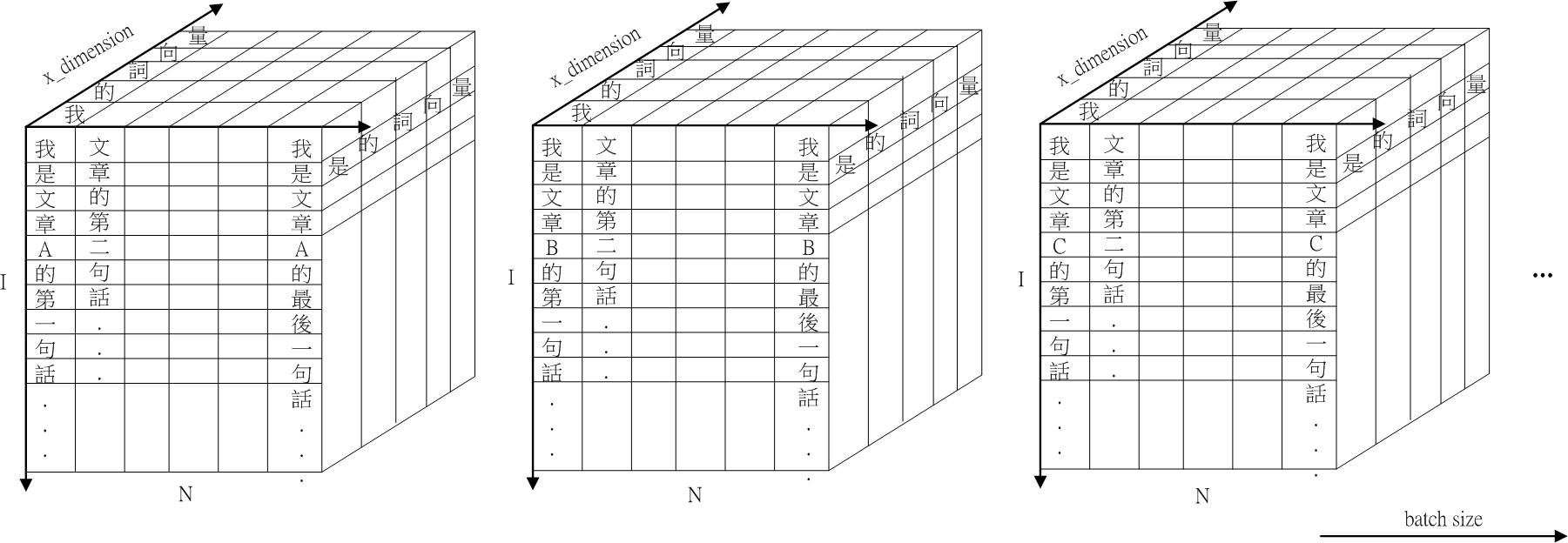Fig.2 self.p 示意圖。

Fig.2 呈現 self.p ($\bar{\bar{P}}$) 的示意圖。self.p 有四個維度：batch size, sentence num ($N$), sentence length ($I$), x_dimension。

假設 paragraph 為N 句話: "我是文章的第一句話...，文章的第二句話...,..., 我是文章的第N句話" 。

每一句話的長度皆為 I。

x_dimension 是 word vector 的長度。

batch_size 是批次的 size。

26行 L2 normalization正規化

26      normal_p = tf.nn.l2_normalize(self.p,3)

26 行將 self.p 的第四個維度 (note 維度從 0 計算，3 則是第四個維度)，x_dimension 維度做 L2 正規化，結果存入 normal_p。

L2 正規化 (L2 normalization，簡稱 L2 norm) 的輸入與輸出都是一個 vector (一維陣列)。

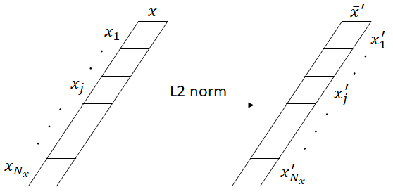
Fig.3 L2 norm 示意圖

Fig.3 為 L2 norm 示意圖。輸入和輸出皆是向量，計算對應的 element $x_j$

假定一個 vector $\bar{x}=[x_1,x_2,\cdots, x_j, \cdots, x_{N_x}]$，其中 $N_x$ 是 $\bar{x}$ 的 element 個數，則 $\bar{x}$ 的 L2 正規化的計算式可表示為：

$x_j'=\frac{x_j}{\displaystyle \sqrt{ \sum_{i=1}^{N_x} x_i^2}}$

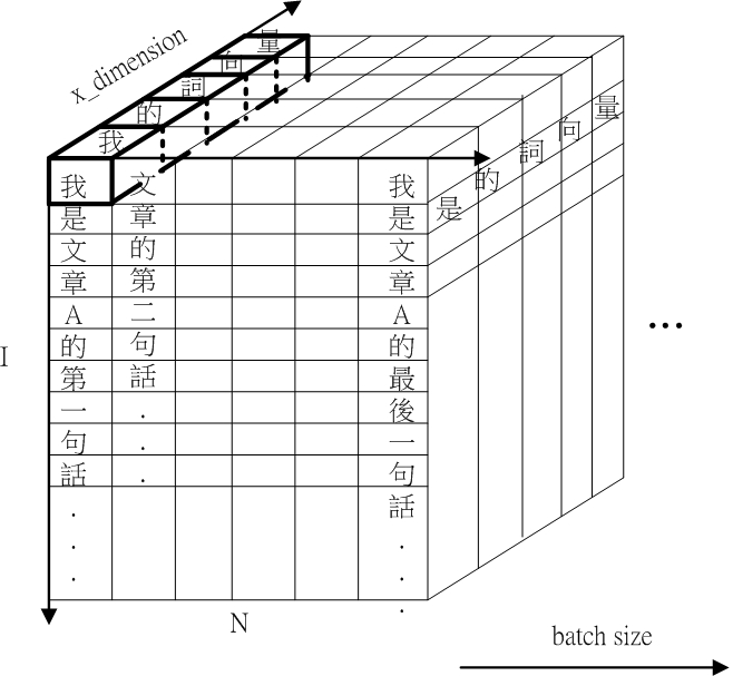
Fig.4 self.p 以 x_dimension 維度計算 L2 norm 的示意圖

Fig.4 呈現self.p ($\bar{\bar{P}}$) 以 x_dimension 維度做 L2 正規化的示意圖。self.p ($\bar{\bar{P}}$) 的每個字向量都進行 L2 norm 計算

27, 28行 Reshape 轉換tensor 形狀

27      ## (batch_size,max_plot_len*max_len[0],x_dimension)
28      normal_p = tf.reshape(normal_p,[batch_size,max_plot_len*max_len[0],x_dimension])

28 行將 $\textrm{normal}\_\textrm{p}$ (四維，$\textrm{batch}\_\textrm{size} \times N \times I \times \textrm{x}\_\textrm{dimension}$) reshape 成三維 $\textrm{batch}\_\textrm{size} \times (N \times I) \times \textrm{x}\_\textrm{dimension}$

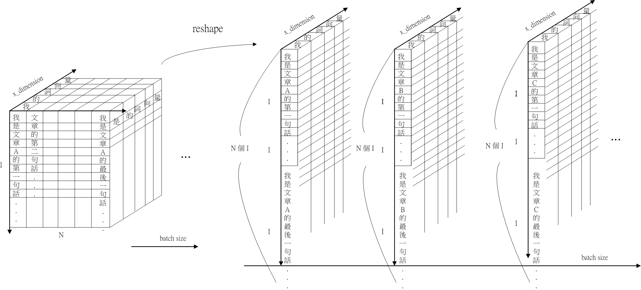Fig.5 schematic of normal p reshape。

fig.5 呈現 normal_p 的示意圖。normal_p reshape 後，N 的 dimension 消失，I 的 dimension 增為 $N \times I$

$\textrm{normal}\_\textrm{p} \in R^{\textrm{batch}\_\textrm{size} \times (\textrm{max}\_\textrm{plot}\_\textrm{len} \times \textrm{max}\_\textrm{len[0]}) \times \textrm{x}\_\textrm{dimension}} = R^{\textrm{batch}\_\textrm{size} \times (N \times I) \times \textrm{x}\_\textrm{dimension}}$

15 行 定義 $\bar{\bar{Q}}$ (Query)

15      self.q = tf.placeholder(shape=(batch_size,max_len[1],x_dimension), dtype=tf.float32) ##(batch_size,q_sentence_length,x_dimension)

15 行將定義一個 tensor self.q，它指的是論文的$\bar{\bar{Q}}$ (query)
$\textrm{self.q} \in R^{\textrm{batch}\_\textrm{size} \times \textrm{max}\_\textrm{len[1]} \times \textrm{x}\_\textrm{dimension}} = R^{\textrm{batch}\_\textrm{size} \times J \times \textrm{x}\_\textrm{dimension}}$。

其中 max_len[1] ($\textrm{J}$) is number of word in a query sentence

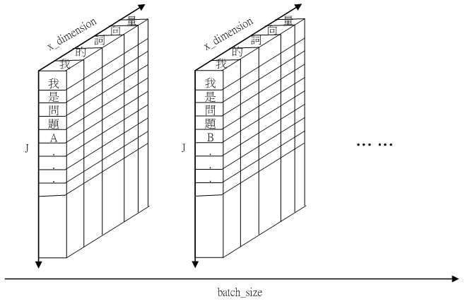
Fig.6 Schematic of self.q

Fig.6 呈現 self.q 的示意圖。self.q 有三個維度：batch size, word number in sentence ( $J$ ), x_dimension。

30      ## (batch_size,max_len[1],x_dimension)
31      normal_q = tf.reshape(tf.nn.l2_normalize(self.q,2),[batch_size,max_len[1],x_dimension])

31 行將 self.q 的第三個維度 (維度從 0 計算，2 則是第三個維度)，x_dimension 維度做 L2 正規化，再 reshape 後存入 normal_q。

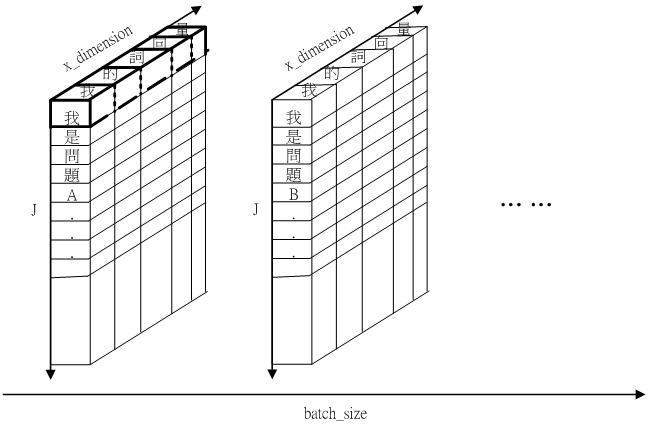
Fig.7 self.q 以 x_dimension 維度計算 L2 norm 的示意圖
Fig.7 呈現self.q 以 x_dimension 維度計算 L2 norm 的示意圖，圖中將
"我"的詞向量(word vector)做L2 norm。

16 行 定義 $\bar{\bar{C}}$ choices

16      self.ans = tf.placeholder(shape=(batch_size*choice,max_len[2],x_dimension), dtype=tf.float32) ##(batch_size*5,ans_sentence_length,x_dimension)

16 行將定義一個 tensor self.ans， $\textrm{self.ans} \in R^{(\textrm{batch}\_\textrm{size} \times \textrm{choice}) \times \textrm{max}\_\textrm{len}[2] \times \textrm{x}\_\textrm{dimension}}$，它就是$\bar{\bar{C}}$ (choice)。

其中，choice 在 main.py 程式中第16行被設定是 5 (number of choices)；

max_len[2] 是$K$ (number of word in a choice)。

$\textrm{self.ans} \in R^{(\textrm{batch}\_\textrm{size} \times \textrm{choice}) \times \textrm{max}\_\textrm{len}[2] \times \textrm{x}\_\textrm{dimension}} = R^{(\textrm{batch}\_\textrm{size} \times 5) \times K \times \textrm{x}\_\textrm{dimension}}$

Fig.8 Schematic of self.ans

Fig.8 呈現 self.ans 的示意圖。self.ans 有三個維度：batch size x 5, word number in sentence ( $K$ ), x_dimension。

33      normal_ans = tf.nn.l2_normalize(self.ans,2)

33 行將 self.ans 的第三個維度 (維度從 0 計算，2 是第三個維度)，x_dimension 維度做 L2 正規化，再 reshape 後存入 normal_ans。

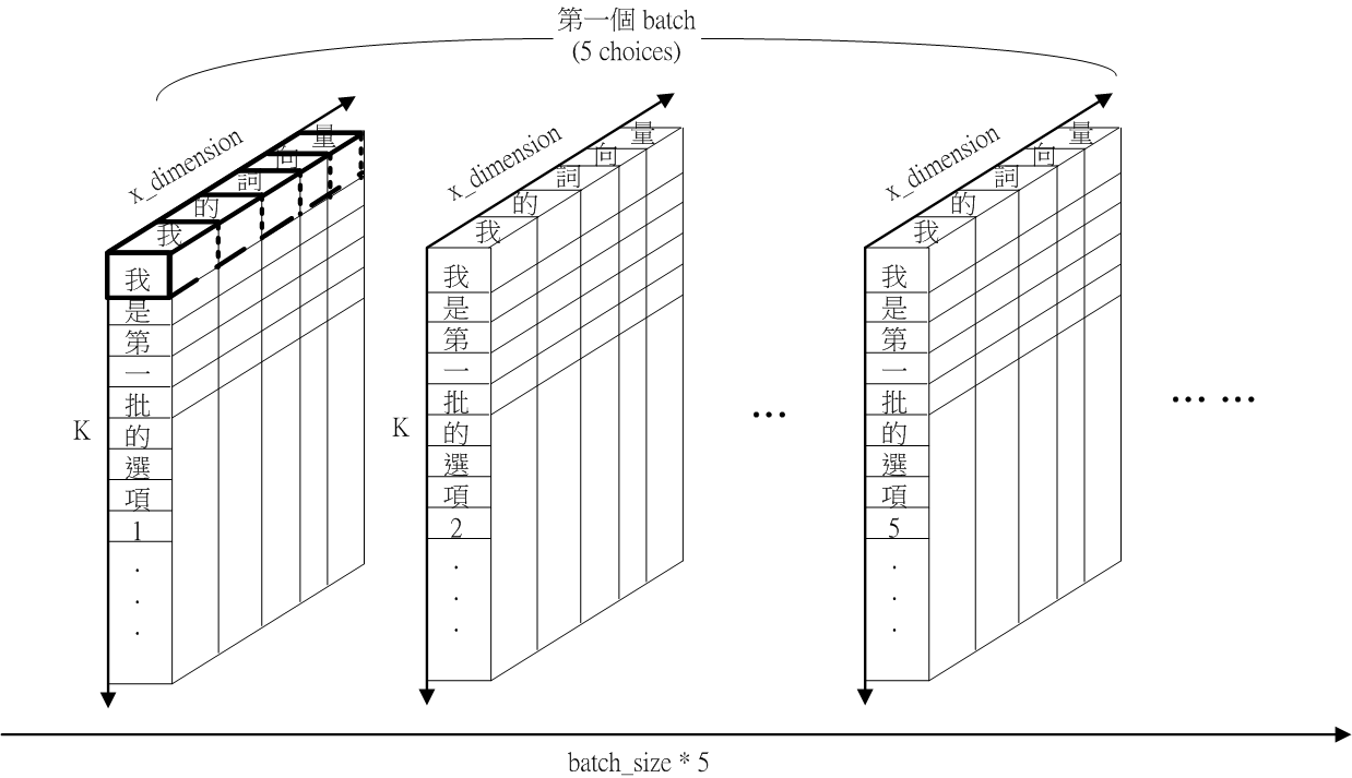
Fig.9 self.ans 以 x_dimension 維度計算 L2 norm 的示意圖

Fig.9 呈現self.ans 以 x_dimension 維度做 L2 正規化。

34      ## (batch_size,choice*max_len[2],x_dimension)
35      normal_ans = tf.reshape(normal_ans,[batch_size,choice*max_len[2],x_dimension])

35 行將 normal_ans，$\textrm{normal}\_\textrm{ans} \in R^{(\textrm{batch}\_\textrm{size} \times \textrm{choice}) \times K \times \textrm{x}\_\textrm{dimension}}$， reshape 成 $\textrm{normal}\_\textrm{ans} \in R^{\textrm{batch}\_\textrm{size} \times (\textrm{choice}\times K) \times \textrm{x}\_\textrm{dimension}}$

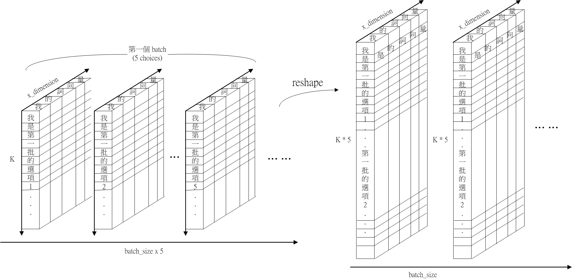
Fig.10 schematic of normal_ans after reshape。

fig.10 呈現 normal_ans 的示意圖。

$\textrm{normal}\_\textrm{ans} \in R^{\textrm{batch}\_\textrm{size} \times (5 \times K) \times \textrm{x}\_\textrm{dimension}}$

​

17行 定義 $\hat{y}$ label data

17      self.y_hat = tf.placeholder(shape=(batch_size,choice), dtype=tf.float32) ##(batch_size,5)

17 行將定義一個 tensor self.y_hat， $\textrm{self.y}\_\textrm{hat} \in R^{\textrm{batch}\_\textrm{size} \times 5}$，它就是 $\hat{y}$ (label data)。

choice = 5 (number of choices)；

18行 定義 dropout rate

18      self.dropoutRate = tf.placeholder(tf.float32)

18 行將定義一個 tensor self.dropoutRate

tf.float32 指 self.dropoutRate 是一個浮點數

19~23行 assign parameters

19      self.filter_size = cnn_filterSize
20      self.filter_size2 = cnn_filterSize2
21      self.filter_num = cnn_filterNum
22      self.filter_num2 = cnn_filterNum2
23      choose_sentence_num = max_plot_len

19 行的 cnn_filterSize 是 width of kernel in CNN1 ($d$).

cnn_filterSize 將在 /main.py 被 assign [1, 3, 5]。

20 行的 cnn_filterSize2 是 width of kernel in CNN2 ($d$).

cnn_filterSize2 將在 /main.py 被 assign [1, 3, 5]。

21 行的 cnn_filterNum 是 number of kernel in CNN1 ($l$).

cnn_filterNum 將在 /main.py 被 assign 128。

22 行的 cnn_filterNum2 是 number of kernel in CNN2 ($l$).

cnn_filterNum2 將在 /main.py 被 assign 128。

23 行的 max_plot_len 是 number of sentence in paragraph $N$

$N$ 將在 /main.py 被 assign 101。

#initialize parameter# 第二部分，Compare layer

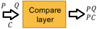
Fig.11 Compare Layer in QACNN model

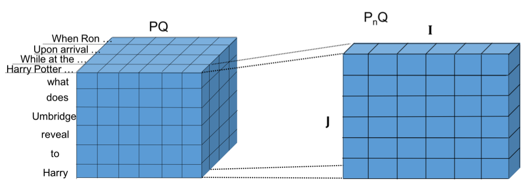Fig.12 Compare layer map between paragraph $\mathbf{P}$ and query $\mathbf{Q}$. $\mathbf{I}$ denotes the length of each sentence $\mathbf{P_n}$, $\mathbf{J}$ denotes the length of query $\mathbf{Q}$.

Fig.12 shows the similarity between paragraph $P$ and query $Q$ . $I$ denotes the length of each sentence $P_n$ .$J$ denotes the length of query $Q$.

$P_{n} Q = \{ \cos (\bar{p}^{i}_{n}, \bar{q}_{j}) \}_{i=1,j=1}^{I,J} = \{ \bar{p}^{i}_{n} \cdot \bar{q}_{j} \}_{i=1,j=1}^{I,J}$

$PQ=[P_1Q,P_2Q,\cdots,P_NQ] \in R^{N \times J \times I}$

__init__() 函數中， # initialize parameters # 第二部分為以下 38~48 行 :

38    PQAttention = tf.matmul(normal_p,tf.transpose(normal_q,[0,2,1])) ##(batch,max_plot_len*max_len[0],max_len[1])
39    PAnsAttention = tf.matmul(normal_p,tf.transpose(normal_ans,[0,2,1])) ##(batch,max_plot_len*max_len[0],choice*max_len[2])
40    PAnsAttention = tf.reshape(PAnsAttention,[batch_size,max_plot_len*max_len[0],choice,max_len[2]]) ##(batch,max_plot_len*max_len[0],choice,max_len[2])
41    PAAttention,PBAttention,PCAttention,PDAttention,PEAttention = tf.unstack(PAnsAttention,axis = 2) ##[batch,max_plot_len*max_len[0],max_len[2]]
42
43    PQAttention = tf.unstack(tf.reshape(PQAttention,[batch_size,max_plot_len,max_len[0],max_len[1],1]),axis = 1) ##[batch,max_len[0],max_len[1],1]
44    PAAttention = tf.unstack(tf.reshape(PAAttention,[batch_size,max_plot_len,max_len[0],max_len[2],1]),axis = 1) ##[batch,max_len[0],max_len[2],1]
45    PBAttention = tf.unstack(tf.reshape(PBAttention,[batch_size,max_plot_len,max_len[0],max_len[2],1]),axis = 1) ##[batch,max_len[0],max_len[2],1]
46    PCAttention = tf.unstack(tf.reshape(PCAttention,[batch_size,max_plot_len,max_len[0],max_len[2],1]),axis = 1) ##[batch,max_len[0],max_len[2],1]
47    PDAttention = tf.unstack(tf.reshape(PDAttention,[batch_size,max_plot_len,max_len[0],max_len[2],1]),axis = 1) ##[batch,max_len[0],max_len[2],1]
48    PEAttention = tf.unstack(tf.reshape(PEAttention,[batch_size,max_plot_len,max_len[0],max_len[2],1]),axis = 1) ##[batch,max_len[0],max_len[2],1]

第38行、43行將計算 paragraph-query similarity map (PQAttention)

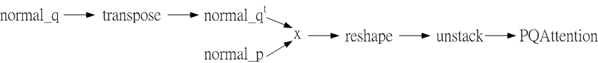fig.13 計算 paragraph-query similarity map (PQAttention) 的流程

fig.13 將執行PQ的計算

$PQ=[P_1Q,P_2Q,\cdots,P_NQ] \in R^{N \times J \times I}$

$P_{n} Q = \{ \cos (\bar{p}^{i}_{n}, \bar{q}_{j}) \}_{i=1,j=1}^{I,J} = \{ \bar{p}^{i}_{n} \cdot \bar{q}_{j} \}_{i=1,j=1}^{I,J}$

其中 PQAttention 是再加上 batch size 維度的 $PQ$

38行 矩陣轉置 (transpose ) 與矩陣相乘 (matmul)

38    PQAttention = tf.matmul(normal_p,tf.transpose(normal_q,[0,2,1])) ##(batch,max_plot_len*max_len[0],max_len[1])

第 38 行的概念是
$\textrm{PQAttention}=\textrm{normal}\_\textrm{p} \times \textrm{normal}\_ \textrm{q}^t$

其中 tf.transpose(normal_q, [0,2,1])，將 normal_q 的維度由 $\textrm{batch} \times J \times \textrm{x}\_\textrm{dimension}$轉成$\textrm{batch} \times \textrm{x}\_\textrm{dimension} \times J$。

Fig.14 normal_q transposation, tf.transpose(normal_q, [0,2,1])

Fig.14 shows normal_q transpose the axis 1 ($J$) and axis 2 (x_dimension).

normal_q 的維度轉置後變成 $\textrm{batch}\_\textrm{size} \times \textrm{x}\_\textrm{dimension} \times J$；

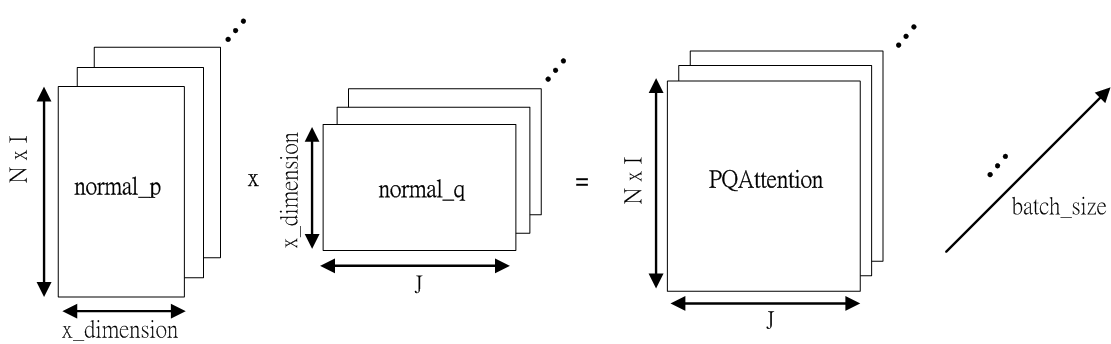Fig.15 normal_p 與 normal_q 矩陣相乘示意圖

normal_p 的維度為 $\textrm{batch}\_\textrm{size} \times (N \times I) \times \textrm{x}\_\textrm{dimension}$；

normal_q 的維度為 $\textrm{batch}\_\textrm{size} \times \textrm{x}\_\textrm{dimension} \times J$；

PQAttention 為 normal_p 與 normal_q 兩矩陣相乘，維度為

$\textrm{batch}\_\textrm{size} \times \left \{ \left[ (N \times I) \times \textrm{x}\_\textrm{dimension} \right ] \left[ \textrm{x}\_\textrm{dimension} \times J \right ] \right \} = \textrm{batch}\_\textrm{size} \times (N \times I) \times J$

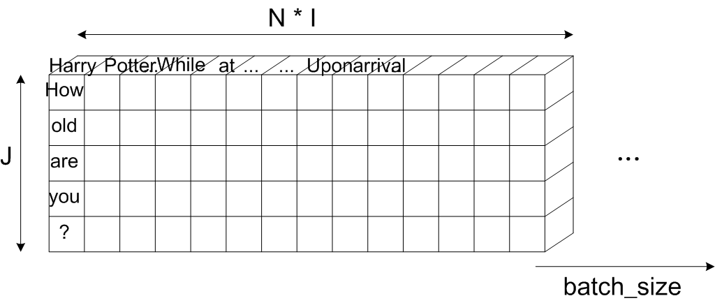
Fig.16 Schematic of PQAttention (multiplied by normal_p and normal_q)

Fig.16 shows the PQAttention after matmul by normal_p and normal_q. The shape of PQAttention is $\textrm{batch}\_\textrm{size} \times (N \times I) \times J$

圖中的第一個column與第一個raw的元素是Harry與how兩個字詞的內積。
圖中的第二個column與第一個raw的元素是Potter與how兩個字詞的內積。
圖中的第一個column與第二個raw的元素是Harry與old兩個字詞的內積。

43行 將PQAttention reshape 與 unstack

43    PQAttention = tf.unstack(tf.reshape(PQAttention,[batch_size,max_plot_len,max_len[0],max_len[1],1]),axis = 1) ##[batch,max_len[0],max_len[1],1]

第 43 行，將 PQAttention reshape 再 unstack。

​

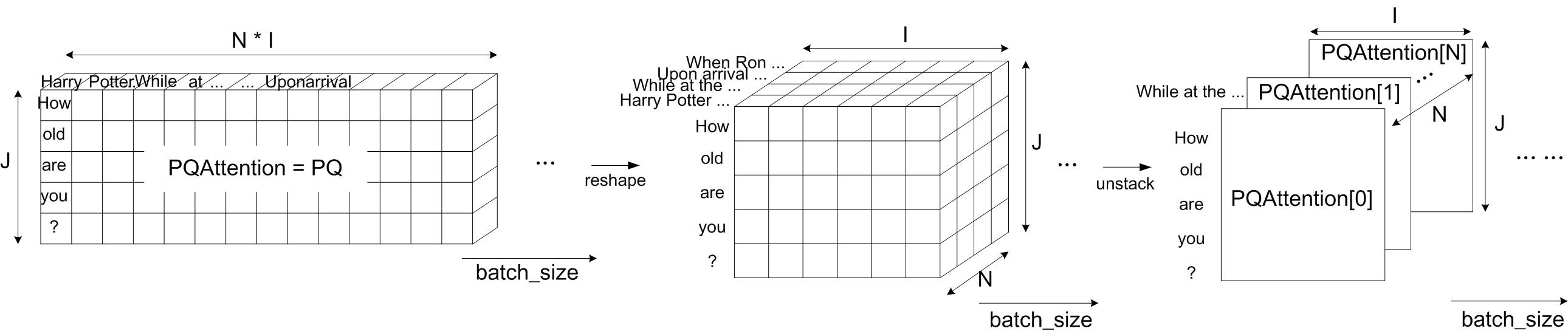
Fig.17 PQAttention shape transformation

Fig.17 呈現將 PQAttention reshape 與 unstack 的示意圖。
PQAttention reshape 後，維度由 $\textrm{batch}\_\textrm{size} \times (N \times I) \times J \times 1$ 變為 $\textrm{batch}\_\textrm{size} \times N \times I \times J \times 1$，

PQAttention unstack 將 PQAttention 內部拆成 N 個矩陣，PQAttention[0] to PQAttention[N-1]。

PQAttention[0] 的維度為 $\textrm{batch}\_\textrm{size} \times I \times J \times 1$

39~40行 PAnsAttention computation

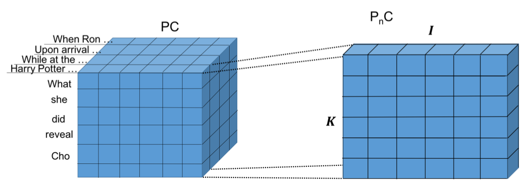
Fig.18 Similarity map between paragraph $P$ and choice $C$. $K$ denotes the length of choice $C$.

Fig.18 shows the similarity between paragraph $P$ and choice $C$ .

Each word in sentences of paragraph is compared to each word in query and choice.

$P_{n}C = \{ \cos \bar{p}_{n}^{i}, \bar{c}_{k} \}_{i=1,j=1}^{I,K}$

The paragraph-choice (PC) similarity map are created as

$PC = [ P_{1}C,P_{2}C,\cdots,P_{N}C] \in R^{N \times K \times I}$

39  PAnsAttention = tf.matmul(normal_p,tf.transpose(normal_ans,[0,2,1])) ## batch,max_plot_len*max_len[0],choice*max_len[2])

39 行將 normal_p 與轉置過後的 normal_ans 相乘，得到 PAnsAttension

normal_p 的維度為 $\textrm{batch}\_\textrm{size} \times (N \times I) \times \textrm{x}\_\textrm{dimension}$；

normal_ans 的維度為 $\textrm{batch}\_\textrm{size} \times (5 \times K) \times \textrm{x}\_\textrm{dimension}$；經過轉置後維度是 $\textrm{batch}\_\textrm{size} \times \textrm{x}\_\textrm{dimension} \times (5 \times K)$

normal_p 乘上 normal_ans 的維度是

$\textrm{batch}\_\textrm{size} \times \left \{ \left[ (N \times I) \times \textrm{x}\_\textrm{dimension} \right ] \left[ \textrm{x}\_\textrm{dimension} \times (5 \times K) \right ] \right \} = \textrm{batch}\_\textrm{size} \times (N \times I) \times (5 \times K)$，存為 PAnsAttention

40  PAnsAttention = tf.reshape(PAnsAttention,[batch_size,max_plot_len*max_len[0],choice,max_len[2]]) ##(batch,max_plot_len*max_len[0],choice,max_len[2])

40 行將 PAnsAttention 從三維 $\textrm{batch}\_\textrm{size} \times (N \times I) \times (5 \times K)$ reshape 成四維 $\textrm{batch}\_\textrm{size} \times (N \times I) \times 5 \times K$

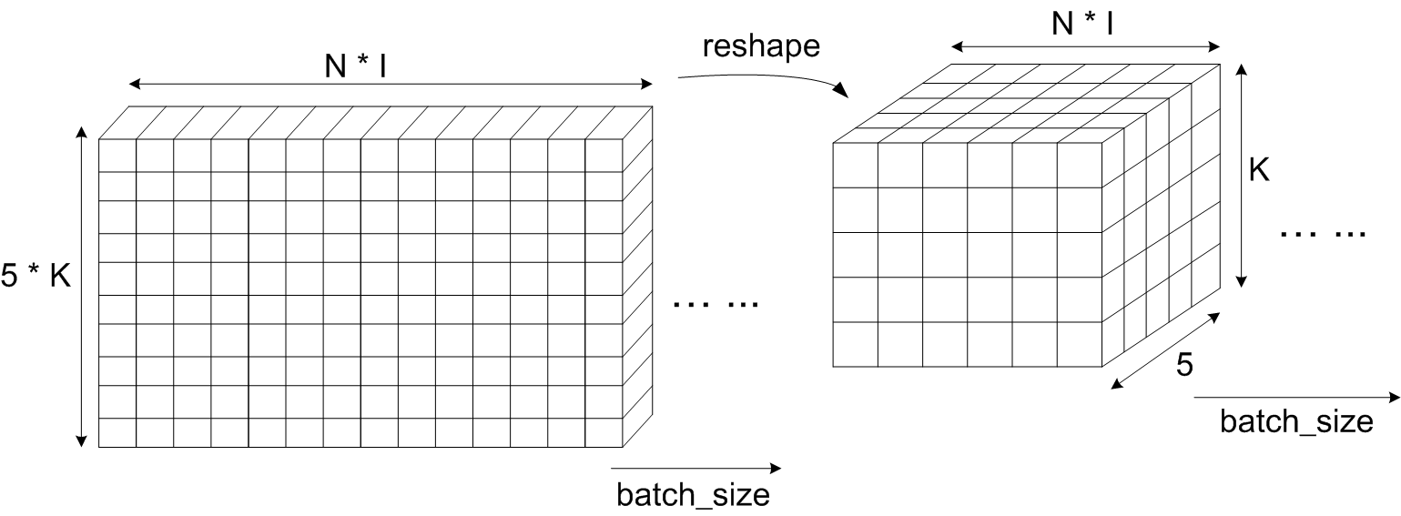Fig.19 PAnsAttention shape transformation

Fig.19 shows the PAnsAttention shape transformation from $\textrm{batch}\_\textrm{size} \times (N \times I) \times (5 \times K)$ to $\textrm{batch}\_\textrm{size} \times (N \times I) \times 5 \times K$

41~44行 PAAttention, PBAttention, ..., PEAttention computation

41  PAAttention,PBAttention,PCAttention,PDAttention,PEAttention = tf.unstack(PAnsAttention,axis = 2) ##[batch,max_plot_len*max_len[0],max_len[2]]
44  PAAttention = tf.unstack(tf.reshape(PAAttention,[batch_size,max_plot_len,max_len[0],max_len[2],1]),axis = 1) ##[batch,max_len[0],max_len[2],1]

41行將 PAnsAttention 以 choice 維度 unstack 為 PAAttention, PBAttention, PCAttention, PDAttention, PEAttention

44行將 PAAttention reshape 後再 unstack。

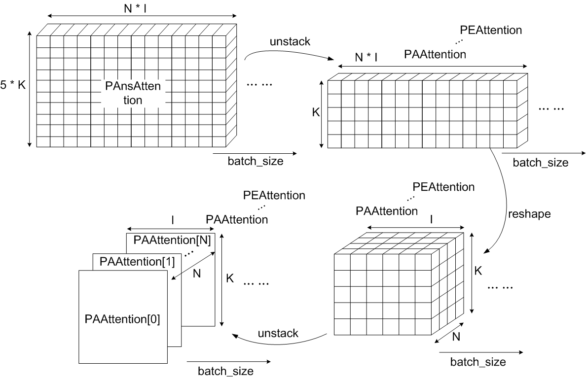Fig.20 PAAttention...PEAttention shape transformation (note. 將N的維度獨立出來)

Fig.20 為 PAnsAttention 經過 41、44行成 PAAttention 的轉換圖。

41 行將 PAnsAttention 以 axis=2 的維度 (choice) unstack，得到 5 個矩陣 (choice=5)，各別存入 PAAttention, PBAttention, PCAttention, PDAttention, PEAttention，維度各別是 $\textrm{batch}\_\textrm{size} \times (N \times I) \times K$

44 行將 PAAttention 的維度 $\textrm{batch}\_\textrm{size} \times (N \times I) \times K$ reshape 為 $\textrm{batch}\_\textrm{size} \times N \times I \times K$，再將 axis=1 的維度 (N) unstack，產生 $N$ 個維度為 $\textrm{batch}\_\textrm{size} \times I \times K$ 的矩陣

45    PBAttention = tf.unstack(tf.reshape(PBAttention,[batch_size,max_plot_len,max_len[0],max_len[2],1]),axis = 1) ##[batch,max_len[0],max_len[2],1]
46    PCAttention = tf.unstack(tf.reshape(PCAttention,[batch_size,max_plot_len,max_len[0],max_len[2],1]),axis = 1) ##[batch,max_len[0],max_len[2],1]
47    PDAttention = tf.unstack(tf.reshape(PDAttention,[batch_size,max_plot_len,max_len[0],max_len[2],1]),axis = 1) ##[batch,max_len[0],max_len[2],1]
48    PEAttention = tf.unstack(tf.reshape(PEAttention,[batch_size,max_plot_len,max_len[0],max_len[2],1]),axis = 1) ##[batch,max_len[0],max_len[2],1]

同理，第 45~48 行的 PBAttention ... PEAttention 維度為 $\textrm{batch}\_\textrm{size} \times I \times K$ 的矩陣。

Reference

[1] tf.nn.l2_normalize https://www.tensorflow.org/api_docs/python/tf/nn/l2_normalize​

[2] tf.nn.l2_normalize的使用 https://blog.csdn.net/abiggg/article/details/79368982​

[3] tf.reshape https://www.tensorflow.org/api_docs/python/tf/reshape​

​

​