QACNN Algorithm

MM 0605/2018

In question answering task, a reading paragraph $P_{\textrm{raw}}$, a query $Q_{\textrm{raw}}$ and several answer choices $C_{\textrm{raw}}$ are given.

The target of the model is to choose a correct answer from multiple choices based on information of $P_{\textrm{raw}}$ and $Q_{\textrm{raw}}$.

Fig.1 Overview on QACNN model. $\bar{y}$ denotes the probability of choices A, B, C and D.

Fig.1 shows the pipeline overview of QACNN.

The embedding layer is used to transform $P_{\textrm{raw}}$, $Q_{\textrm{raw}}$, $C_{\textrm{raw}}$ into word embedding $P$, $Q$, $C$.

The compare layer generates paragraph-query similarity map $PQ$ and paragraph-choice similarity map $PC$.

The QACNN consists of two staged-CNN architecture.

The first stage projects word level feature into sentence-level, and the second stage projects sentence-level feature into paragraph-level.

The output of first stage are paragraph's sentence features based on the query $\bar{\bar{r}}^{PQ}$ and choice $\bar{\bar{r}}^{PC}$

$\bar{\bar{r}}^{PQ}=[\bar{r}^{PQ}_1,\cdots, \bar{r}^{PQ}_n, \cdots,\bar{r}^{PQ}_N]$ and $\bar{\bar{r}}^{PC}=[\bar{r}^{PC}_1,\cdots, \bar{r}^{PC}_n, \cdots,\bar{r}^{PC}_N]$.

$n$ is the index for sentence, and $N$ is the total number of sentence in paragraph.

The output of second stage is answer feature $\bar{r}$.

Each choice has its corresponding answer feature.

Every choice answer feature, $\bar{r}_A$, $\bar{r}_B$, $\bar{r}_C$, $\bar{r}_D$, are inputs to prediction layer, and the output denotes the probability of choices A, B, C and D, respectively.

$\bar{y}=[p_A,p_B,p_C,p_D]$.

Similarity Mapping layer

Similarity mapping layer is composed of two part $\colon$ embedding layer and compare layer.

Given a paragraph $P_{\textrm{raw}}$ (with $N$ sentences), a query $Q_{\textrm{raw}}$, and a choice $C_{\textrm{raw}}$, the embedding layer transforms every words in $P_{\textrm{raw}}$, $Q_{\textrm{raw}}$ and $C_{\textrm{raw}}$ into word embedding $\colon$
$P =\{\bar{p}_n^i \}_{i=1,n=1}^{I,N}$ $\colon$ $N$ is the total number of sentence in paragraph, and $I$ is the total number of words in each sentence.

$Q =\{\bar{q}^j \}_{j=1}^{J}$ $\colon$ Query is considered as one sentence.

$C = \{ \bar{c}^k \}_{k=1}^K$ $\colon$ choice is considered as one sentence.

The sentences in all the paragraphs have the same length by padding.

$J$ is the total number of words in query sentence. $K$ is the total number of words in choice sentence.

$\bar{p}_n^i$, $\bar{q}^j$ and $\bar{c}^k$ are word embeddings.

Word embedding can be obtained by any type of embedding technique, such as RNN, sequence-to-sequence model, Word2Vec, etc.

The pre-trained Glo Ve word vectors is adopted as the embedding without further modification [3].

The compare layer compares each paragraph sentence $P_n$ to $Q$ and $C$ at word level separately.

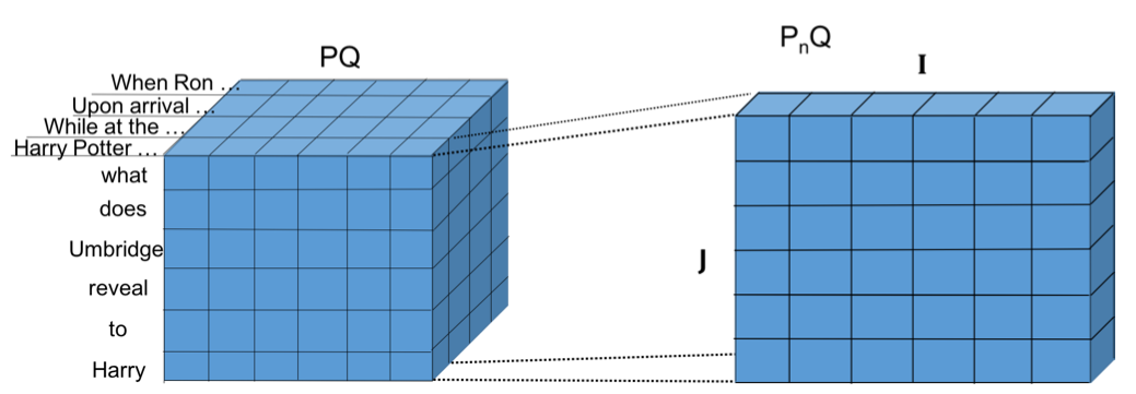
Fig.2 Similarity map between paragraph $\mathbf{P}$ and query $\mathbf{Q}$. $\mathbf{I}$ denotes the length of each sentence $\mathbf{P_n}$, $\mathbf{J}$ denotes the length of query $\mathbf{Q}$.

Fig.2 shows the similarity between paragraph $P$ and query $Q$. $I$ denotes the length of each sentence $P_n$. $J$ denotes the length of query $Q$. $P_{n}Q = {\{ \cos \left(\bar{p}_n^i,\bar{q}^j \right) \}}_{i=1,j=1}^{I,J}$

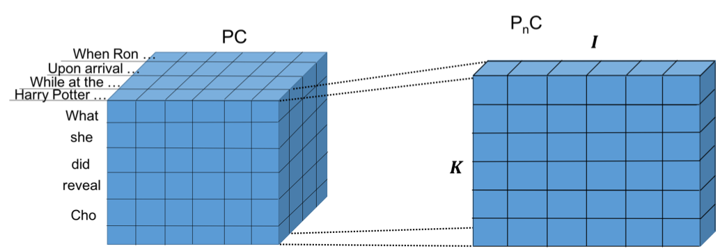Fig.3 Similarity map between paragraph $P$ and choice $C$. $K$ denotes the length of choice $C$.

Fig.3 shows the similarity between paragraph $P$ and choice $C$. $K$ denotes the total number of words in choice sentence $C$.

Each word in sentences of paragraph is compared to each word in query and choice.

$P_{n}C={\{ \cos (\bar{p}_n^i,\bar{c}^k) \}}_{i=1,k=1}^{I,K}$

Two similarity map, paragraph-query ($PQ$) and paragraph-choice ($PC$) similarity map are created as

$PQ=[P_{1}Q,P_{2}Q, \cdots ,P_{N}Q] \in R^{N \times J \times I}$

$PC=[P_{1}C,P_{2}C, \cdots ,P_{N}C] \in R^{N \times K \times I}$

QACNN Layer

QACNN contains a two-staged CNN combined with query-based attention mechanism.

An attention convolutional matching layer is used to integrate two similarity maps.

QACNN layer is used to learn the location relationship pattern.

Each stage comprises two major part$\colon$ attention map and output representation.

Attention Map of First stage

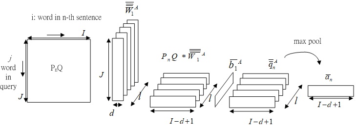
Fig.4-0 First stage CNN attention part, from $P_nQ$ to word-level attention map $\bar{a}_n$.

Fig. 4-0 shows the derivation of word-level attention map $\bar{a}_n$ from $P_nQ$.

$P_n Q \in R^{J \times I}$ is $n$-th sentence slice $P_n Q \in R^{J \times I}$in $PQ$ , and CNN is applied on $P_nQ$ with convolution kernel $\bar{\bar{\bar{W}}}_1^A \in R^{J \times l \times d}$ . $d$ and $l$ represent width of kernel and number of kernel, respectively.

The superscript $A$ denotes attention map, and the subscript $1$ denotes the first stage CNN.

The generated feature $\bar{\bar{q}}_n^A \in R^{l \times(I-d+1)}$ is expressed as

$\bar{\bar{q}}_n^A =\textrm{sigmoid}( \bar{\bar{W}}_1^A * P_n Q + \bar{b}_1^A)$

where $\bar{b}_1^A \in R^l$ is the bias.

With $\bar{\bar{W}}_1^A$ would learn the query syntactic structure and give weight to each paragraph's location. Sigmoid function is chosen as activation function in this stage.

Max pooling is performed to $\bar{\bar{q}}_n^A$ perpendicularly to find the largest weight between different kernels in the same location, using max pool kernel shaped $l$, and then generate word-level attention map $\bar{a}_n \in R^{I-d+1}$ for each sentence.

$\bar{a}_n = \textrm{max pool}(\bar{\bar{q}}_n^A)$, note $\bar{\bar{q}}_n^A \in R^{l \times (I-d+1)}$ and $\bar{a}_n \in R^{I-d+1}$.

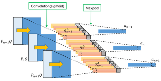
Fig.4 First stage CNN attention part. Each paragraph sentences are used to generate its corresponding word-level attention map $\bar{a}_n$, $n=1,2,\cdots,N$.

Fig.4 shows the architecture of the attention map in first stage CNN, and all sentences in paragraph are used.

Output Representation of First Stage

The paragraph's sentence features based on the query ($\bar{\bar{r}}^{PQ}$) and the choice ($\bar{\bar{r}}^{PC}$) are derived at first stage.

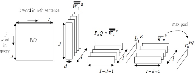
Fig.5-0 Derivation of paragraph feature based on query, $\bar{r}_n^{PQ}$.

Fig.5-0 shows the derivation of paragraph feature based on query, $\bar{r}_n^{PQ}$.

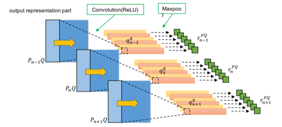
Fig.5 All paragraph's sentence feature based on query, $\bar{\bar{r}}^{PQ}=[\bar{r}_1^{PQ},\cdots,\bar{r}_n^{PQ},\cdots,\bar{r}_N^{PQ}]$.

Fig.5 shows all paragraph's sentence feature based on query, $\bar{\bar{r}}^{PQ}=[\bar{r}_1^{PQ},\cdots,\bar{r}_n^{PQ},\cdots,\bar{r}_N^{PQ}]$.

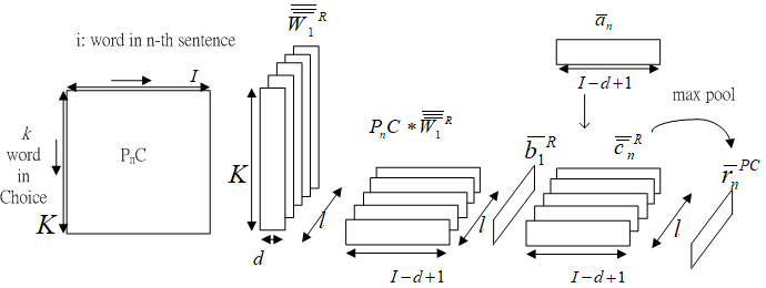
Fig.6-0 Derivation of paragraph's sentence feature based on choice, $\bar{r}_n^{PC}$.

Fig.6-0 shows the derivation of paragraph's sentence feature based on choice, $\bar{r}_n^{PC}$.

.

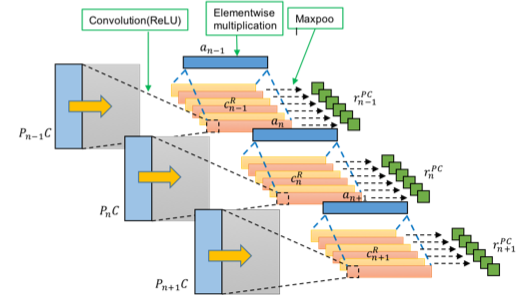
Fig.6 All paragraph's sentence feature based on choice, $\bar{\bar{r}}^{PC}=[\bar{r}_1^{PC},\cdots,\bar{r}_n^{PC},\cdots,\bar{r}_N^{PC}]$.

Fig.6 shows all paragraph's sentence feature based on choice, $\bar{\bar{r}}^{PC}=[\bar{r}_1^{PC},\cdots,\bar{r}_n^{PC},\cdots,\bar{r}_N^{PC}]$.

$\bar{\bar{r}}^{PQ}$ and $\bar{\bar{r}}^{PC}$ are two output representation part of first-stage CNN architecture.

Kernels $\bar{\bar{\bar{W}}}_1^R \in R^{l \times K \times d}$ and bias $\bar{b}_1^R \in R^l$ are applied to $P_n Q$ to acquire query-based sentence features.

$\bar{\bar{q}}_n^R = \textrm{ReLU}(\bar{\bar{\bar{W}}}_1^R \otimes P_n Q + \bar{b}_1^R) \in R^{l \times ( I-d+1)}$

Identical kernels $\bar{\bar{\bar{W}}}_1^R \in R^{l \times K \times d}$ and bias $\bar{b}_1^R \in R^l$ are applied to $P_n C$ to aggregate pattern of location relationship and acquire choice-based sentence features. The superscript $R$ denotes output representation

$\bar{\bar{c}}_n^R = \textrm{ReLU}(\bar{\bar{\bar{W}}}_1^R \otimes P_n C + \bar{b}_1^R)= \left[ \begin{matrix} (\bar{c}_{n,1}^R)^t \\ \vdots \\(\bar{c}_{n,\ell}^R)^t \end{matrix} \right] \in R^{l \times ( I-d+1)}$

$\bar{\bar{c}}_n^R$ is multiplied by the word-level attention map $\bar{a}_n \in R^{I-d+1}$ through the first dimension.

$\bar{\bar{c}}_n^R=\left[ \begin{matrix} (\bar{c}_{n,1}^R)^t \odot \bar{a}_n \\ \vdots \\(\bar{c}_{n,\ell}^R)^t \odot \bar{a}_n \end{matrix} \right]$,

The max pool operations are applied on $\bar{\bar{q}}_n^R \in R^{l \times ( I-d+1)}$ and $\bar{\bar{c}}_n^R \in R^{l \times ( I-d+1)}$ horizontally with kernel shape $(I-d+1)$ to get the query-based sentence features $\bar{r}_n^{PQ} \in R^l$ and choice-based sentence features $\bar{r}_n^{PC} \in R^l$.

$\bar{r}_n^{PQ} = \textrm{max pool}(\bar{\bar{q}}_n^R)$

$\bar{r}_n^{PC} = \textrm{max pool}(\bar{\bar{c}}_n^R)$

Attention map of second stage

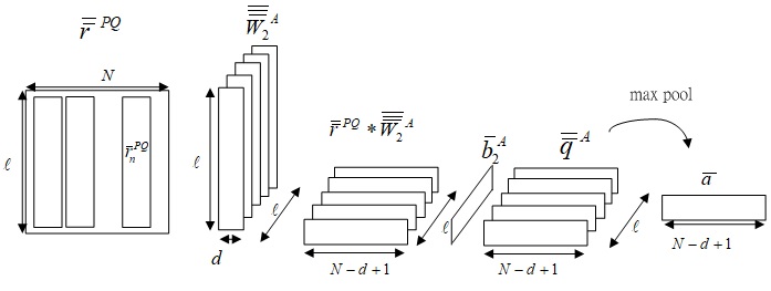
Fig.7-0 Derivation of sentence-level attention map $\bar{a}$ from $\bar{\bar{r}}^{PQ}$.

Fig.7-0 shows the derivation of sentence-level attention map $\bar{a}$ from query-based sentence features $\bar{\bar{r}}^{PQ}$.

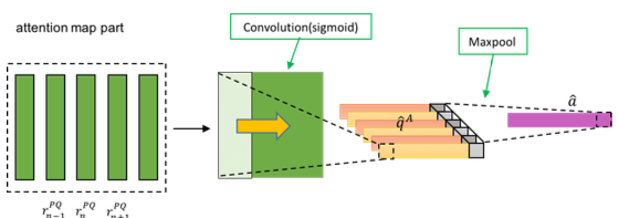
Fig.7 Derivation of sentence-level attention map $\bar{a}$ from $\bar{\bar{r}}^{PQ}$.

Fig.7 shows the derivation of sentence-level attention map $\bar{a}$ from query-based sentence features $\bar{\bar{r}}^{PQ}$.

$\bar{\bar{r}}^{PQ}=[\bar{r}_1^{PQ}, \bar{r}_2^{PQ}, \cdots, \bar{r}_N^{PQ}]$ is the input of second stage CNN, and will be further refined by CNN with kernel $\bar{\bar{\bar{W}}}_2^A \in R^{l \times d \times l}$ and generates intermediate features $\bar{\bar{q}}^A \in R^{l \times N-d+1}$.

$\bar{\bar{q}}^A=\textrm{sigmoid}(\bar{\bar{\bar{W}}}_2^A* \bar{\bar{r}}^{PQ} + \bar{b}_2^A)$

The max pool operation is applied on $\bar{\bar{q}}^A$ with kernel shaped $l$, and the sentence-level attention map $\bar{a} \in R^{N-d+1}$ is obtained.

$\bar{a}=\textrm{max pool}(\bar{\bar{q}}^A)$

Output Representation of Second Stage

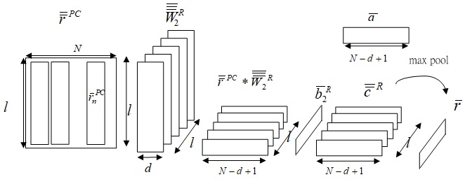
Fig.8-0 Derivation of answer feature $\bar{r}$ from $\bar{\bar{r}}^{PC}$.

Fig. 8-0 shows the derivation of answer feature $\bar{r}$ from $\bar{\bar{r}}^{PC}$.

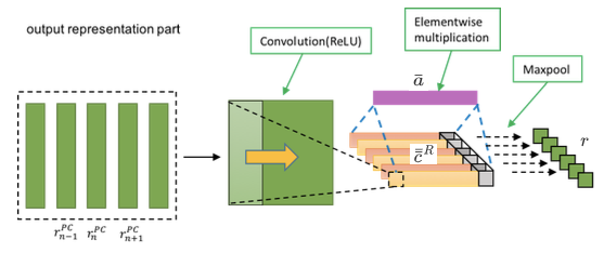
Fig.8 Derivation of answer feature $\bar{r}$ from choice-based sentence feature $\bar{\bar{r}}^{PC}$ .

Fig.8 shows the output representation part of the second stage.

The output representation part of the second stage has two input$\colon$ sentence-level attention map $\bar{a}$ and sentence-level features $\bar{\bar{r}}^{PC}=[\bar{r}_1^{PC},\bar{r}_2^{PC},\bar{r}_N^{PC} ]$.

The $\bar{\bar{c}}^R$ and answer feature $\bar{r}$ is obtained as

$\bar{r}=\{ \textrm{max} (c_t^R \odot a)\}_{t=1}^l$

where

$\bar{\bar{c}}^R = \textrm{ReLU}(\bar{\bar{\bar{W}}}_2^R*\bar{\bar{r}}^{PC} + \bar{b}_2^R)$

and $\bar{\bar{\bar{W}}}_2^R \in R^{l \times l \times d}$, $\bar{b}_2^R \in R^l$, and $\bar{\bar{c}}^R \in R^{l \times (N-d+1)}$. The output representation of certain choice $\bar{r} \in R^l$ is the final output of QACNN Layer.

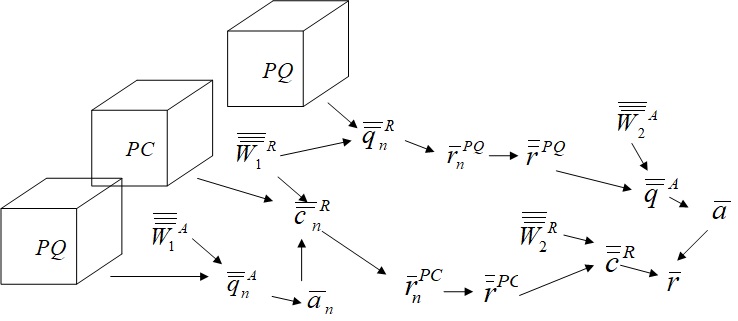
Fig.9 Overall data flow of QACNN.

Prediction Layer

Prediction layer is the final part of QACNN. $\bar{r}_A \in R^l$ is used to represent the final output representation of the $A$-th choice.

$\bar{r}_A, \bar{r}_B, \bar{r}_C, \bar{r}_D$ is passed to two-fully-connected layer and compute probability for each choice using softmax

$\bar{\bar{R}} =[\bar{r}_A, \bar{r}_B, \bar{r}_C, \bar{r}_D]$.

The output vector is the probability of each choices

$\bar{y} = \left[ \begin{matrix} p_A \\ p_B \\ \vdots \\ p_E \end{matrix} \right] = \textrm{softmax}(\bar{\bar{W}}^o(\textrm{tanh}( \bar{\bar{W}}^p \bar{\bar{R}} + \bar{b}^p )) + b^o)$.

where $\bar{\bar{W}}^p \in R^{l \times l}$, $\bar{b}^p \in R^l$, $\bar{\bar{W}}^o \in R^{l \times M_c}$ and $b^o \in R^{M_c}$.

Two fully-connected layer are applied.

$\bar{\bar{W}}^P$ and $\bar{\bar{W}}^o$ are the weight matrix of first and second fully-connected layer, respectively.

$\bar{b}^p$ and $\bar{b}^o$ are the bias of first and second fully-connected layer, respectively.

$M_c$ is the number of choices.

Hyperbolic function can be expressed as

$\textrm{tanh} x = \frac{e^x-e^{-x}}{e^x + e^{-x}}$.

[0]

Query-based Attention CNN for Text Similarity Map

Tzu-Chien Liu, Yu-Hsueh Wu, Hung-Yi Lee, 2017.

[1]

M.Tapaswi, Y.Zhu, R. Stiefelhagen,

"Movieqa: Understanding stories in movies through question-answering," IEEE Conference on Computer Vision and Pattern Recognition (CVPR), 2016.

[2]

oS. Wang and J. Jiang, " A compare-aggregate model for matching text sequences," 1611.01747, 2016.

[3]

J. Pennington, R. Socher, and C. Manning, "Glove: Global vectors for word representation," in Proceedings of the 2014 conference on empirical methods in natural language processing (EMNLP), 2014, pp.1532-1543.